Topic 4 Portfolio Concepts MeanVariance Analysis Meanvariance portfolio

Topic 4: Portfolio Concepts

Mean-Variance Analysis • Mean–variance portfolio theory is based on the idea that the value of investment opportunities can be meaningfully measured in terms of mean return and variance of return.

Assumptions of the Model 1. All investors are risk averse; they prefer less risk to more for the same level of expected return. 2. Expected returns for all assets are known. 3. The variances and covariances of all asset returns are known. 4. Investors need only know the expected returns, variances, and covariances of returns to determine optimal portfolios. 5. There are no transaction costs or taxes.

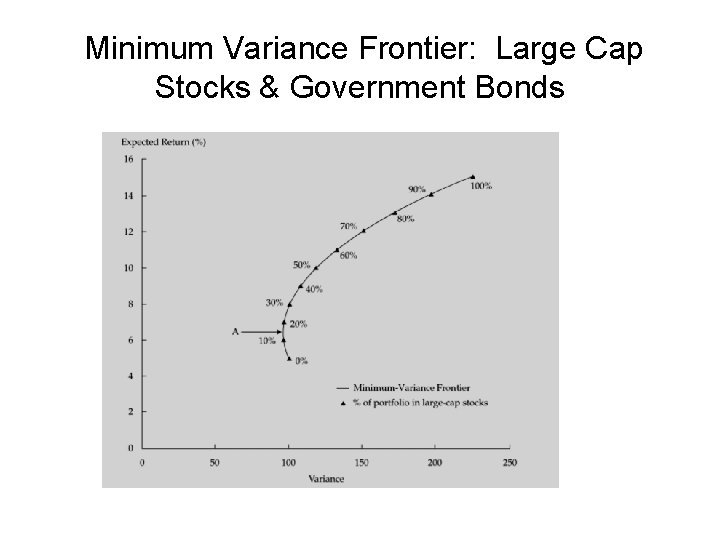
Minimum Variance Frontier • An investor’s objective in using a mean– variance approach to portfolio selection is to choose an efficient portfolio. – An efficient portfolio is one offering the highest expected return for a given level of risk as measured by variance or standard deviation of return. – Portfolios that have the smallest variance for each given level of expected return are called minimum-variance portfolios.

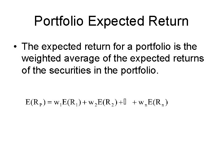
Portfolio Expected Return • The expected return for a portfolio is the weighted average of the expected returns of the securities in the portfolio.

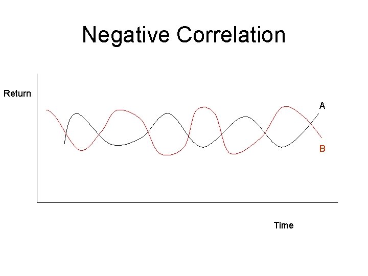
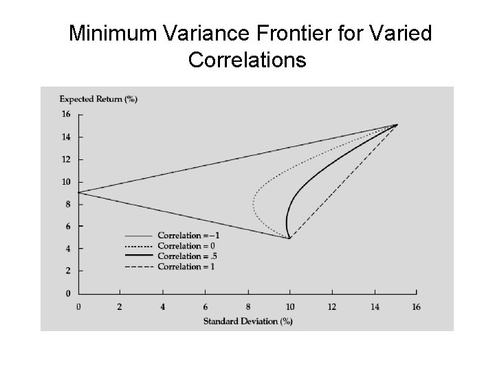
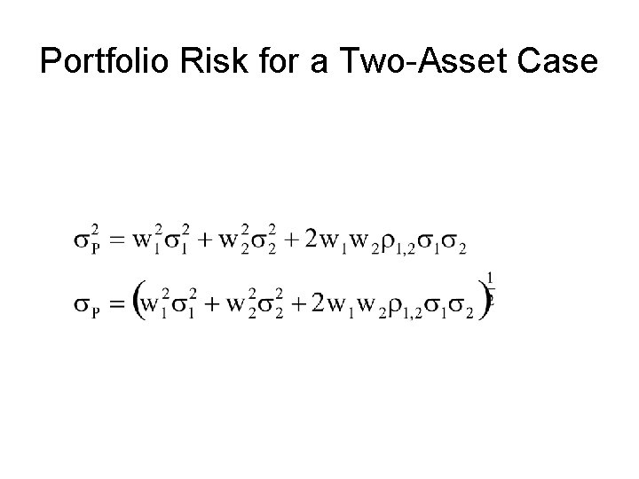
Portfolio Variance • Although it might seem reasonable for the variance of a portfolio to be the weighted average of the variances of the securities in the portfolio, this is incorrect. • Portfolio variance consists of the variances of the individual securities, but must also consist of a factor that measures the interaction of each pair of securities. • Intuitively, if two risky securities are held in a portfolio, but Security A tends to do well when Security B does poorly, and vice versa, a portfolio of the two securities will have less risk. – we can account for the relationship between each pair of securities by using the covariance or the correlation. – Even though both assets are risky, a combination of the two will create a portfolio that is less risky than each of its components. • If we plot two assets in risk/expected return space we get :

Negative Correlation Return A B Time

Minimum Variance Frontier: Large Cap Stocks & Government Bonds

Minimum Variance Frontier for Varied Correlations

Portfolio Risk for a Two-Asset Case

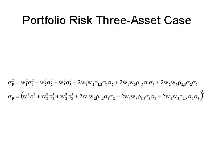
Portfolio Risk Three-Asset Case

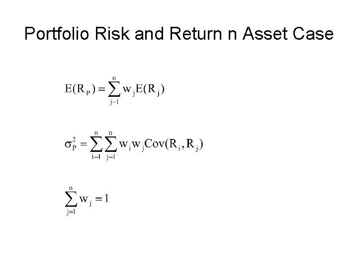
Portfolio Risk and Return n Asset Case

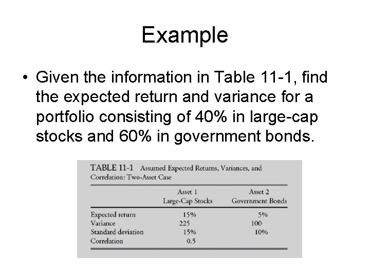
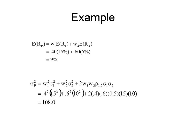
Example • Given the information in Table 11 -1, find the expected return and variance for a portfolio consisting of 40% in large-cap stocks and 60% in government bonds.

Example

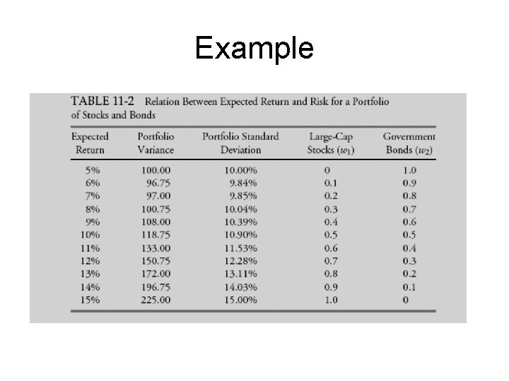
Example • We can find the expected return and variance for portfolios with different combinations of our two assets. Table 112 shows the different expected returns and risk for various portfolios.

Example

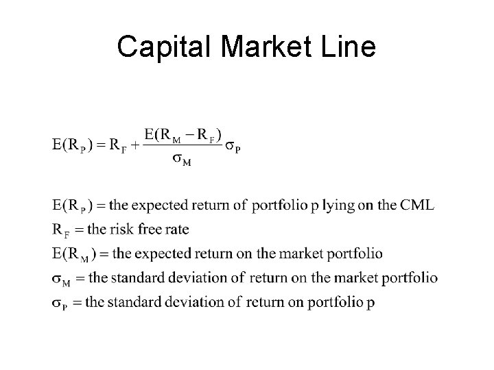
Capital Market Line

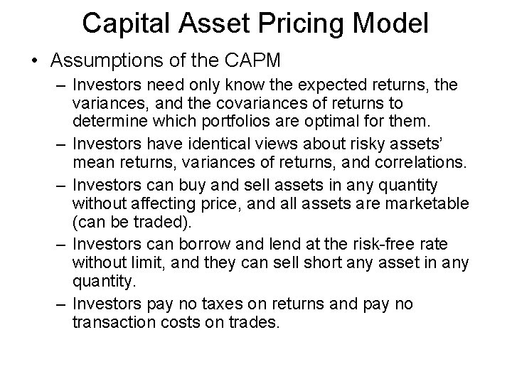
Capital Asset Pricing Model • Assumptions of the CAPM – Investors need only know the expected returns, the variances, and the covariances of returns to determine which portfolios are optimal for them. – Investors have identical views about risky assets’ mean returns, variances of returns, and correlations. – Investors can buy and sell assets in any quantity without affecting price, and all assets are marketable (can be traded). – Investors can borrow and lend at the risk-free rate without limit, and they can sell short any asset in any quantity. – Investors pay no taxes on returns and pay no transaction costs on trades.

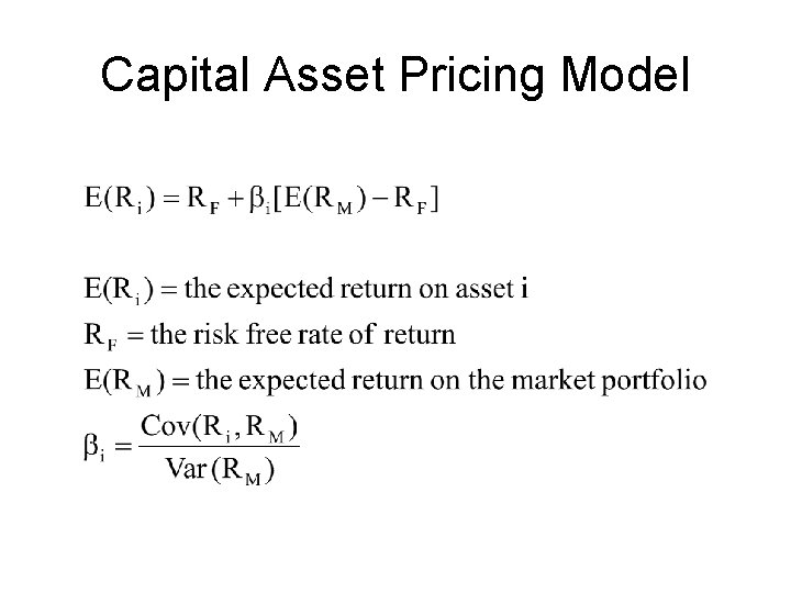
Capital Asset Pricing Model

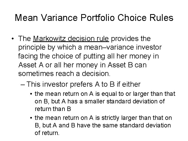
Mean Variance Portfolio Choice Rules • The Markowitz decision rule provides the principle by which a mean–variance investor facing the choice of putting all her money in Asset A or all her money in Asset B can sometimes reach a decision. – This investor prefers A to B if either • the mean return on A is equal to or larger than that on B, but A has a smaller standard deviation of return than B • the mean return on A is strictly larger than that on B, but A and B have the same standard deviation of return.

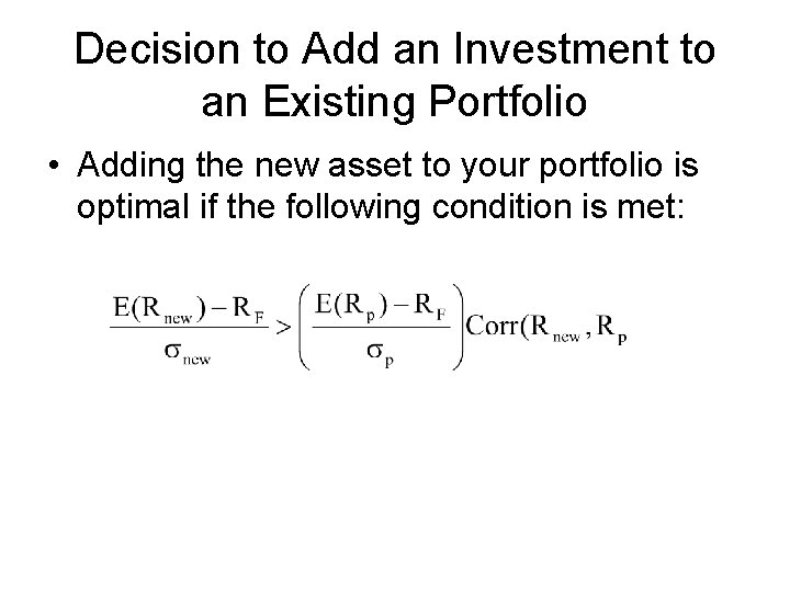
Decision to Add an Investment to an Existing Portfolio • Adding the new asset to your portfolio is optimal if the following condition is met:

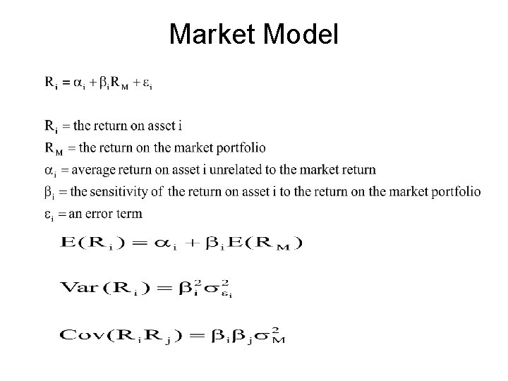
Market Model

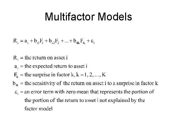
Multifactor Models

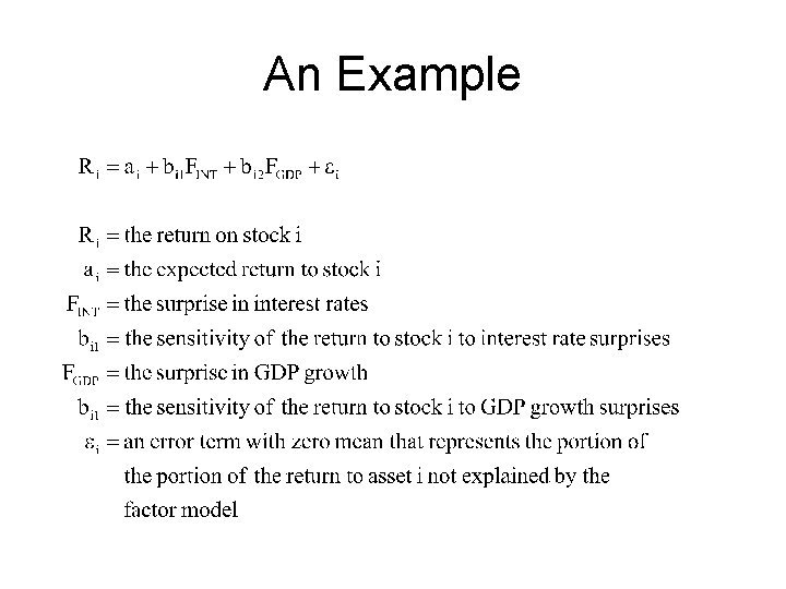
An Example

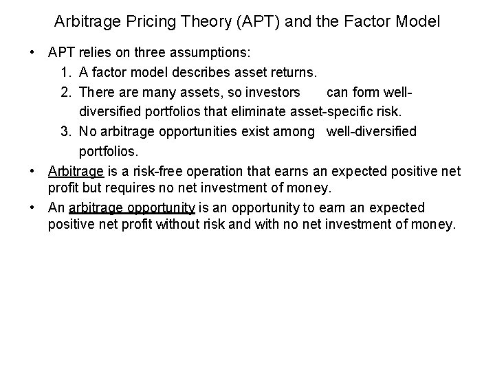
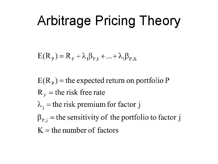
Arbitrage Pricing Theory (APT) and the Factor Model • APT relies on three assumptions: 1. A factor model describes asset returns. 2. There are many assets, so investors can form welldiversified portfolios that eliminate asset-specific risk. 3. No arbitrage opportunities exist among well-diversified portfolios. • Arbitrage is a risk-free operation that earns an expected positive net profit but requires no net investment of money. • An arbitrage opportunity is an opportunity to earn an expected positive net profit without risk and with no net investment of money.

Arbitrage Pricing Theory

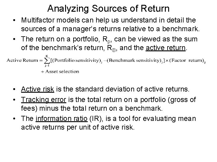
Analyzing Sources of Return • Multifactor models can help us understand in detail the sources of a manager’s returns relative to a benchmark. • The return on a portfolio, Rp, can be viewed as the sum of the benchmark’s return, RB, and the active return. • Active risk is the standard deviation of active returns. • Tracking error is the total return on a portfolio (gross of fees) minus the total return on a benchmark. • The information ratio (IR), is a tool for evaluating mean active returns per unit of active risk.

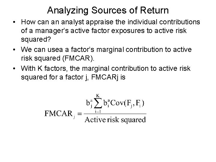
Analyzing Sources of Return • How can an analyst appraise the individual contributions of a manager’s active factor exposures to active risk squared? • We can usea a factor’s marginal contribution to active risk squared (FMCAR). • With K factors, the marginal contribution to active risk squared for a factor j, FMCARj is

Creating a Tracking Portfolio • In a risk-controlled active or enhanced index strategy, the portfolio manager may attempt to earn a small incremental return relative to the benchmark while controlling risk by matching the factor sensitivities of the portfolio to her benchmark. • A tracking portfolio is a portfolio having factor sensitivities that are matched to those of a benchmark or other portfolio.