Topic 3 A General Model of Pollution Control

Topic 3 A General Model of Pollution Control 1

Learning Objectives After this topic you should be able to Understand that a trade-off exists between environmental damages and pollution abatement costs Illustrate and explain the notion of marginal damage functions and why they are useful Illustrate and explain the notion of marginal abatement functions Illustrate and evaluate the social efficient level of pollution emissions Apply the equi-marginal principle to the problem of pollution control 2

First, some important questions • What is the appropriate level of environmental quality we ought to try and achieve? • How do we allocate reductions in emissions over many polluters? • How are benefits and costs of environmental programs distributed across society? 3

Pollution Control: Our Simple Model • Pollution Control: Two Aspects • Damages • Abatement Costs • In general the greater the level of pollution the greater the level of damages and the greater the abatement costs 4

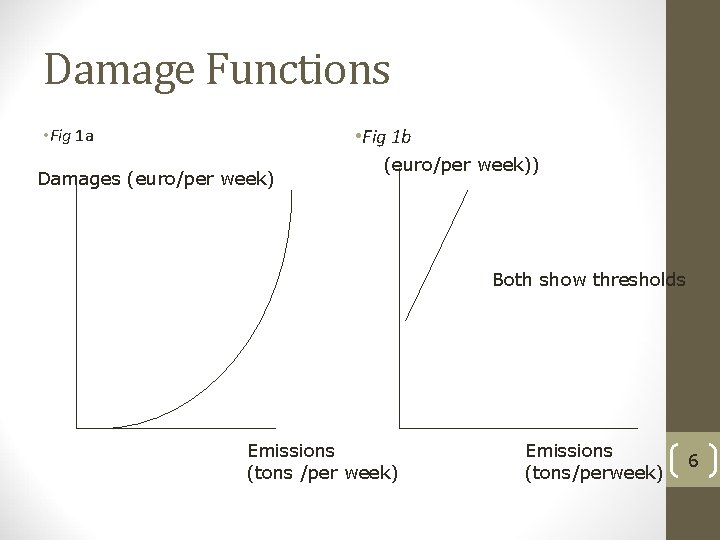
Damage Functions • A damage function describes the relationship between pollution and damage • A marginal damage function shows the changes in damages stemming from a one unit change in emissions or ambient concentrations • The height and shape of a damage function depends on the pollutant and circumstances involved 5

Damage Functions • Fig 1 b • Fig 1 a Damages (euro/per week)) Both show thresholds Emissions (tons /per week) Emissions (tons/perweek) 6

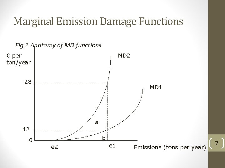
Marginal Emission Damage Functions Fig 2 Anatomy of MD functions € per ton/year MD 2 28 MD 1 a 12 0 b e 2 e 1 Emissions (tons per year) 7

Damage Functions • Two emission damage functions shown • Consider MD 1 and MD 2 • What are marginal damages at e 1? • What are total damages at e 1? • What is the difference between the two functions? • What causes the MD function to shift? • Population change • Different time horizon 8

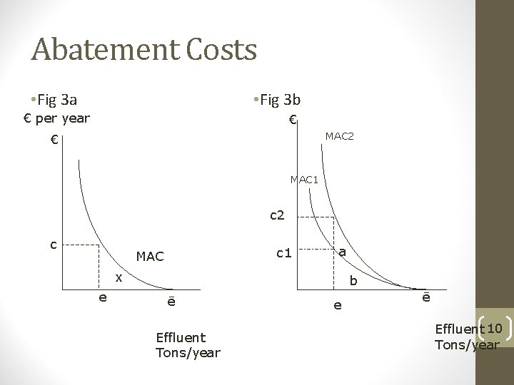
Abatement Costs • Costs of reducing the quantities of residuals being emitted or of lowering ambient concentrations • Marginal abatement cost functions are the costs associated with lowering emitted residuals by one unit • Quantities of pollution on the horizontal axis • Monetary value on vertical axis • Marginal Costs must be read from right to left • The origin = uncontrolled emission levels (ē) 9

Abatement Costs • Fig 3 a • Fig 3 b € per year € MAC 2 € MAC 1 c 2 c c 1 MAC a x e b ē Effluent Tons/year e ē Effluent 10 Tons/year

Marginal Abatement Costs • MAC 1 lies below MAC 2 • What are the marginal costs associated with an emission level e? • What are the total abatement costs associated with MAC 1 and MAC 2? • What might cause MAC to shift right or left • Different production technology • Technology change 11

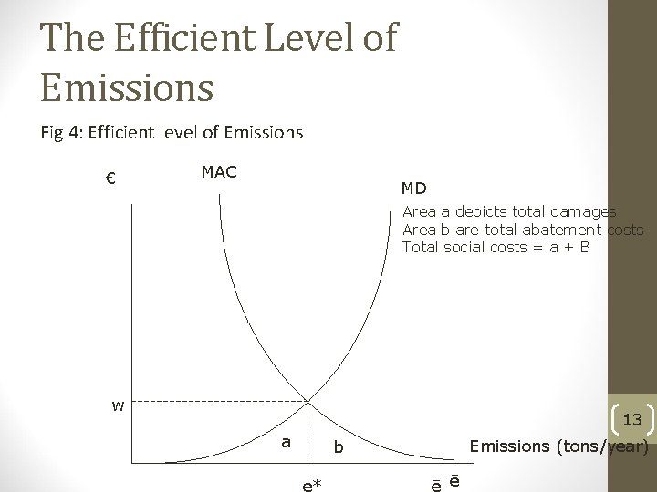
Socially Efficient Level of Emissions • To complete the model and find the socially efficient level of emissions we need to bring together the marginal damage functions and marginal abatement costs • The socially efficient level of emissions is where these are equal • At this point social costs are minimised • There is a trade off between the two • Does this make sense? 12

The Efficient Level of Emissions Fig 4: Efficient level of Emissions € MAC MD Area a depicts total damages Area b are total abatement costs Total social costs = a + B w 13 a Emissions (tons/year) b e* ē ē

Socially Efficient levels of emissions • What causes the MD function to shift? • Population changes • If MD shifts to the right or left what happens to the socially efficient emission levels? • What causes the MAC to shift? • Technology • What happens to e* of this occurs? • Implications for public policy? 14

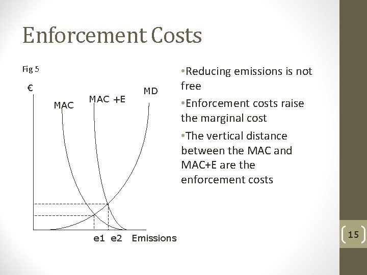
Enforcement Costs Fig 5 € MAC +E MD e 1 e 2 Emissions • Reducing emissions is not free • Enforcement costs raise the marginal cost • The vertical distance between the MAC and MAC+E are the enforcement costs 15

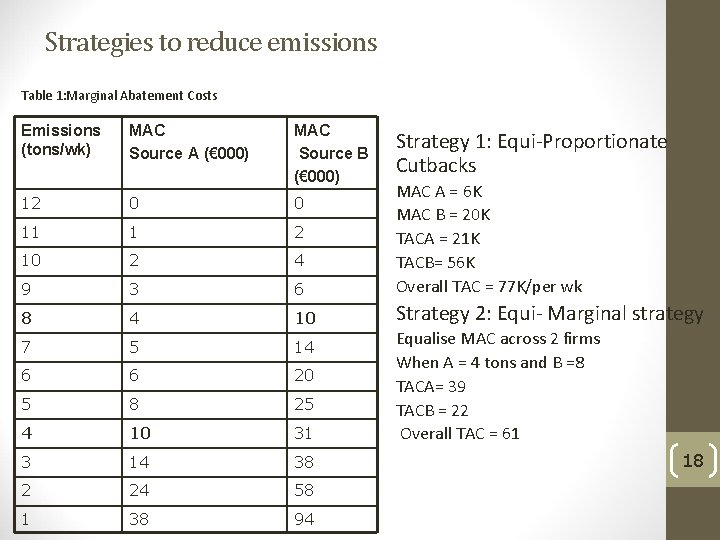
The Equi-Marginal Principle • If there are multiple sources of particular type of pollutant with differing marginal abatement costs and if it is desired to reduce aggregate emissions at the least possible cost, then emissions from the various sources must be reduced in accordance with the equi-marginal principle • Example- see Table 1 16

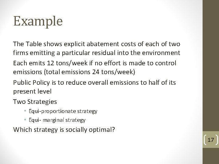
Example The Table shows explicit abatement costs of each of two firms emitting a particular residual into the environment Each emits 12 tons/week if no effort is made to control emissions (total emissions 24 tons/week) Public Policy is to reduce overall emissions to half of its present level Two Strategies • Equi-proportionate strategy • Equi- marginal strategy Which strategy is socially optimal? 17

Strategies to reduce emissions Table 1: Marginal Abatement Costs Emissions (tons/wk) MAC Source A (€ 000) MAC Source B (€ 000) 12 0 0 11 1 2 10 2 4 9 3 6 MAC A = 6 K MAC B = 20 K TACA = 21 K TACB= 56 K Overall TAC = 77 K/per wk 8 4 10 Strategy 2: Equi- Marginal strategy 7 5 14 6 6 20 5 8 25 4 10 31 3 14 38 2 24 58 1 38 94 Strategy 1: Equi-Proportionate Cutbacks Equalise MAC across 2 firms When A = 4 tons and B =8 TACA= 39 TACB = 22 Overall TAC = 61 18

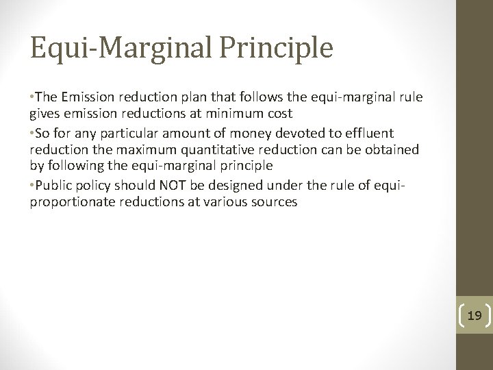
Equi-Marginal Principle • The Emission reduction plan that follows the equi-marginal rule gives emission reductions at minimum cost • So for any particular amount of money devoted to effluent reduction the maximum quantitative reduction can be obtained by following the equi-marginal principle • Public policy should NOT be designed under the rule of equiproportionate reductions at various sources 19

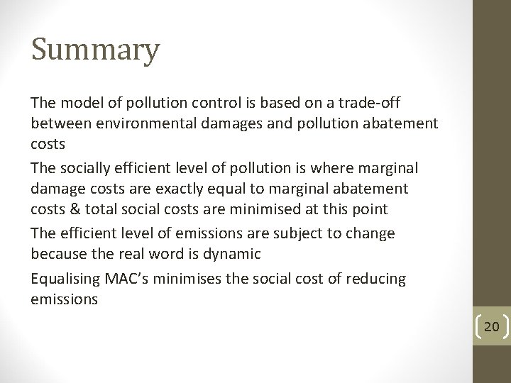
Summary The model of pollution control is based on a trade-off between environmental damages and pollution abatement costs The socially efficient level of pollution is where marginal damage costs are exactly equal to marginal abatement costs & total social costs are minimised at this point The efficient level of emissions are subject to change because the real word is dynamic Equalising MAC’s minimises the social cost of reducing emissions 20

Required Reading • Field & Field, Environmental Economics: An Introduction, chapter 5 21