Topic 17 Interaction Models Interaction Models With several

Topic 17: Interaction Models

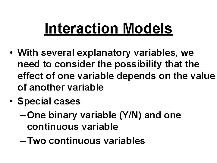
Interaction Models • With several explanatory variables, we need to consider the possibility that the effect of one variable depends on the value of another variable • Special cases – One binary variable (Y/N) and one continuous variable – Two continuous variables

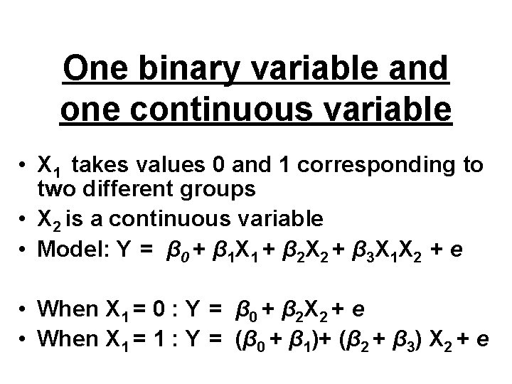
One binary variable and one continuous variable • X 1 takes values 0 and 1 corresponding to two different groups • X 2 is a continuous variable • Model: Y = β 0 + β 1 X 1 + β 2 X 2 + β 3 X 1 X 2 + e • When X 1 = 0 : Y = β 0 + β 2 X 2 + e • When X 1 = 1 : Y = (β 0 + β 1)+ (β 2 + β 3) X 2 + e

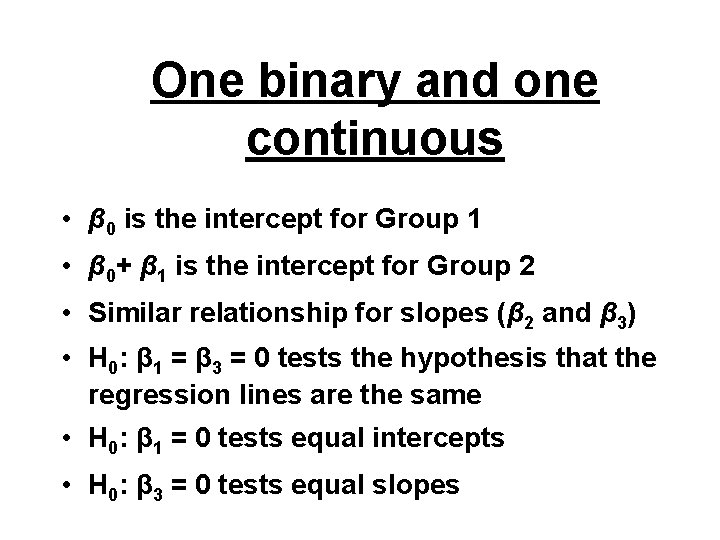
One binary and one continuous • β 0 is the intercept for Group 1 • β 0+ β 1 is the intercept for Group 2 • Similar relationship for slopes (β 2 and β 3) • H 0: β 1 = β 3 = 0 tests the hypothesis that the regression lines are the same • H 0: β 1 = 0 tests equal intercepts • H 0: β 3 = 0 tests equal slopes

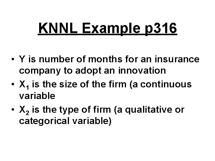
KNNL Example p 316 • Y is number of months for an insurance company to adopt an innovation • X 1 is the size of the firm (a continuous variable • X 2 is the type of firm (a qualitative or categorical variable)

The question • X 2 takes the value 0 if it is a mutual fund firm and 1 if it is a stock fund firm • We ask whether or not stock firms adopt the innovation slower or faster than mutual firms • We ask the question across all firms, regardless of size

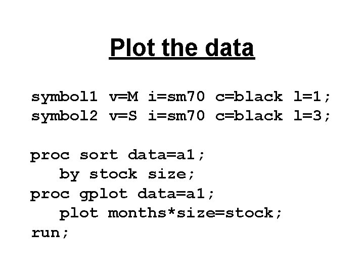
Plot the data symbol 1 v=M i=sm 70 c=black l=1; symbol 2 v=S i=sm 70 c=black l=3; proc sort data=a 1; by stock size; proc gplot data=a 1; plot months*size=stock; run;

Two symbols on plot

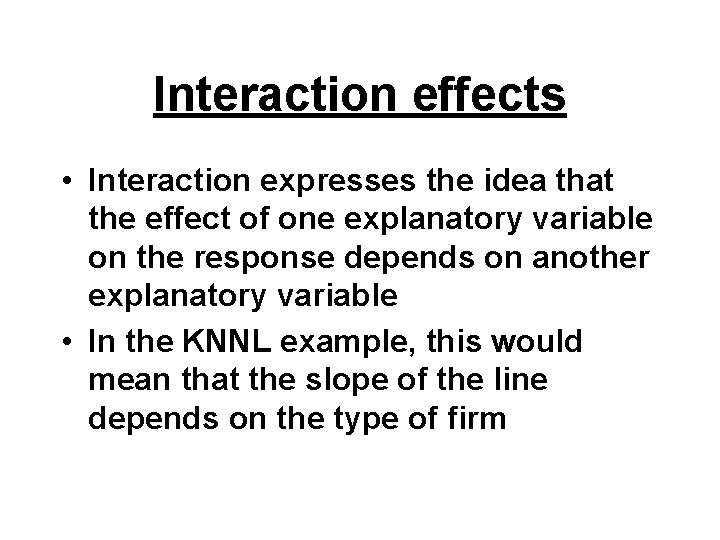
Interaction effects • Interaction expresses the idea that the effect of one explanatory variable on the response depends on another explanatory variable • In the KNNL example, this would mean that the slope of the line depends on the type of firm

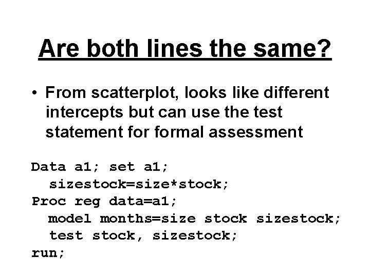
Are both lines the same? • From scatterplot, looks like different intercepts but can use the test statement formal assessment Data a 1; set a 1; sizestock=size*stock; Proc reg data=a 1; model months=size stock sizestock; test stock, sizestock; run;

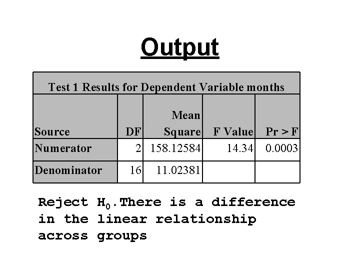
Output Test 1 Results for Dependent Variable months Source Numerator Denominator Mean DF Square 2 158. 12584 16 11. 02381 F Value 14. 34 Pr > F 0. 0003 Reject H 0. There is a difference in the linear relationship across groups

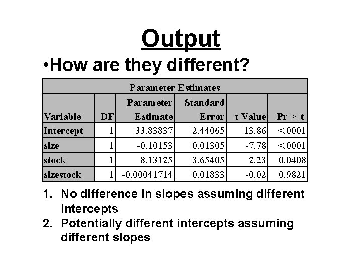
Output • How are they different? Parameter Estimates Variable Intercept size stock sizestock DF 1 1 Parameter Estimate 33. 83837 -0. 10153 8. 13125 -0. 00041714 Standard Error 2. 44065 0. 01305 3. 65405 0. 01833 t Value 13. 86 -7. 78 2. 23 -0. 02 Pr > |t| <. 0001 0. 0408 0. 9821 1. No difference in slopes assuming different intercepts 2. Potentially different intercepts assuming different slopes

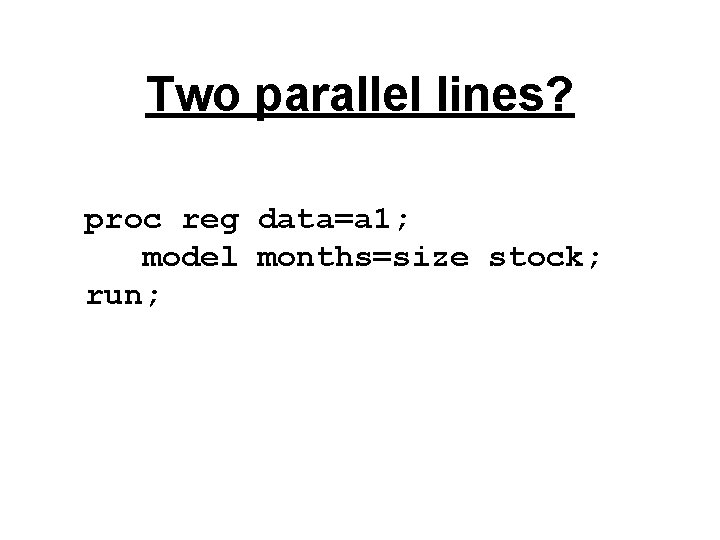
Two parallel lines? proc reg data=a 1; model months=size stock; run;

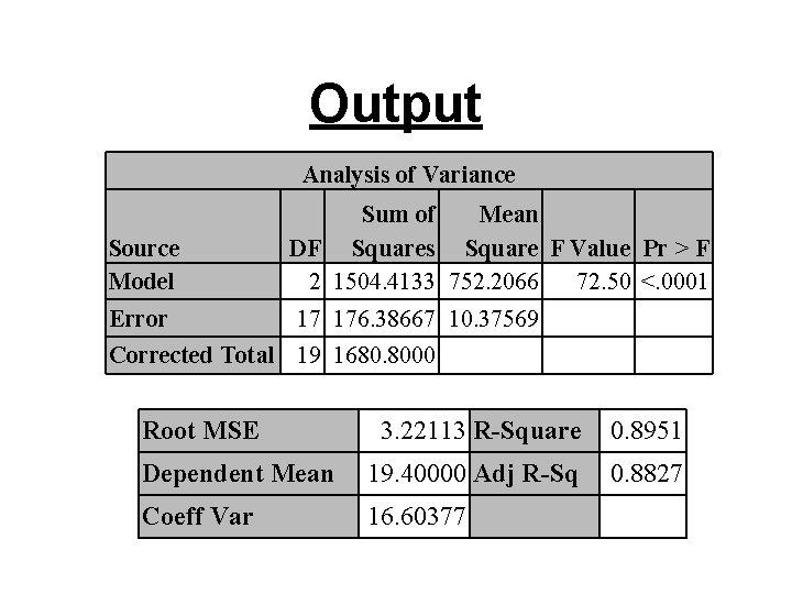
Output Analysis of Variance Source Model Error Sum of Mean DF Squares Square F Value Pr > F 2 1504. 4133 752. 2066 72. 50 <. 0001 17 176. 38667 10. 37569 Corrected Total 19 1680. 8000 Root MSE 3. 22113 R-Square 0. 8951 Dependent Mean 19. 40000 Adj R-Sq 0. 8827 Coeff Var 16. 60377

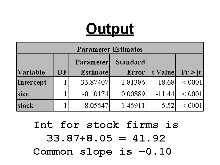
Output Parameter Estimates Variable Intercept DF 1 Parameter Standard Estimate Error t Value Pr > |t| 33. 87407 1. 81386 18. 68 <. 0001 size 1 -0. 10174 0. 00889 -11. 44 <. 0001 stock 1 8. 05547 1. 45911 5. 52 <. 0001 Int for stock firms is 33. 87+8. 05 = 41. 92 Common slope is – 0. 10

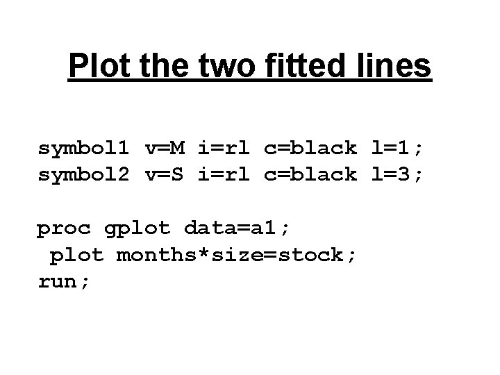
Plot the two fitted lines symbol 1 v=M i=rl c=black l=1; symbol 2 v=S i=rl c=black l=3; proc gplot data=a 1; plot months*size=stock; run;

The plot

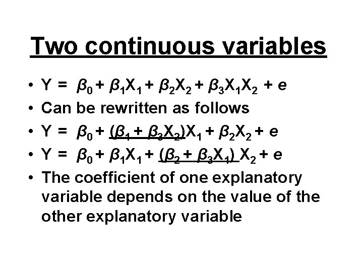
Two continuous variables • • • Y = β 0 + β 1 X 1 + β 2 X 2 + β 3 X 1 X 2 + e Can be rewritten as follows Y = β 0 + (β 1 + β 3 X 2)X 1 + β 2 X 2 + e Y = β 0 + β 1 X 1 + (β 2 + β 3 X 1) X 2 + e The coefficient of one explanatory variable depends on the value of the other explanatory variable

Last slide • We went over KNNL 8. 2 – 8. 7 • We used programs Topic 17. sas to generate the output for today