Topic 11 Lecture 17 Variation and mutation Variation

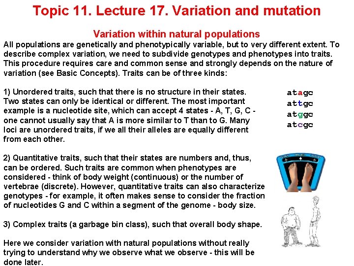
Topic 11. Lecture 17. Variation and mutation Variation within natural populations All populations are genetically and phenotypically variable, but to very different extent. To describe complex variation, we need to subdivide genotypes and phenotypes into traits. This procedure requires care and common sense and strongly depends on the nature of variation (see Basic Concepts). Traits can be of three kinds: 1) Unordered traits, such that there is no structure in their states. Two states can only be identical or different. The most important example is a nucleotide site, which can accept 4 states - A, T, G, C one cannot usually say that A is more similar to T than to G. Many loci are unordered traits, if we all their alleles are equally different from each other. 2) Quantitative traits, such that their states are numbers and, thus, can be ordered. Such traits are common when phenotypes are considered - think of body weight (continuous) or the number of vertebrae (discrete). However, quantitative traits can also characterize genotypes - for example, it often makes sense to consider the fraction of nucleotides G and C within a segment of the genome - body size. 3) Complex traits (a garbage bin class), such that overall body shape. Here we consider variation with natural populations without really trying to understand why we observe what we observe - this will be done later. atagc attgc atggc atcgc

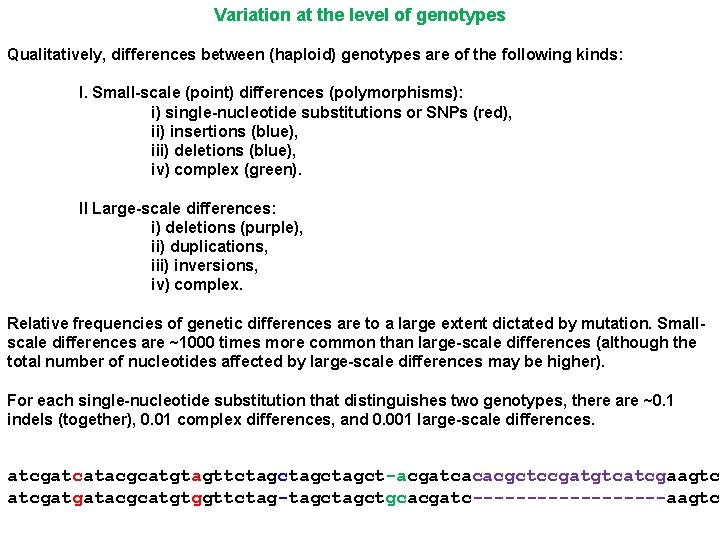
Variation at the level of genotypes Qualitatively, differences between (haploid) genotypes are of the following kinds: I. Small-scale (point) differences (polymorphisms): i) single-nucleotide substitutions or SNPs (red), ii) insertions (blue), iii) deletions (blue), iv) complex (green). II Large-scale differences: i) deletions (purple), ii) duplications, iii) inversions, iv) complex. Relative frequencies of genetic differences are to a large extent dictated by mutation. Smallscale differences are ~1000 times more common than large-scale differences (although the total number of nucleotides affected by large-scale differences may be higher). For each single-nucleotide substitution that distinguishes two genotypes, there are ~0. 1 indels (together), 0. 01 complex differences, and 0. 001 large-scale differences. atcgatcatacgcatgtagttctagctagct-acgatcacacgctccgatgtcatcgaagtc atcgatgatacgcatgtggttctag-tagctgcacgatc---------aagtc

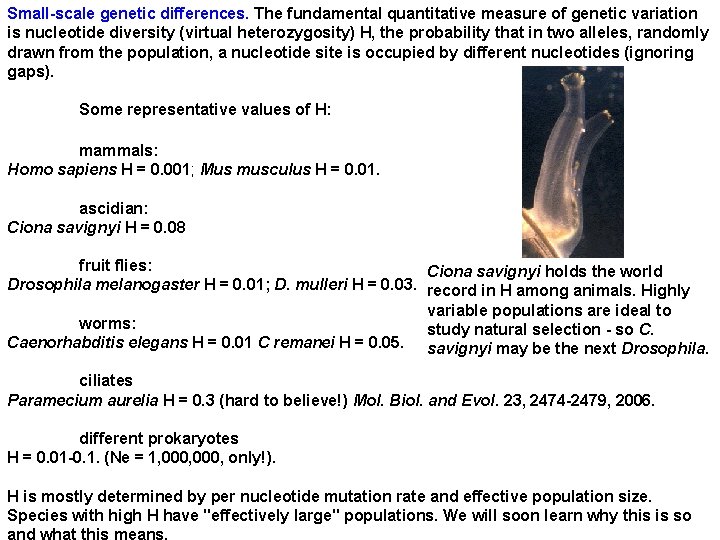
Small-scale genetic differences. The fundamental quantitative measure of genetic variation is nucleotide diversity (virtual heterozygosity) H, the probability that in two alleles, randomly drawn from the population, a nucleotide site is occupied by different nucleotides (ignoring gaps). Some representative values of H: mammals: Homo sapiens H = 0. 001; Mus musculus H = 0. 01. ascidian: Ciona savignyi H = 0. 08 fruit flies: Ciona savignyi holds the world Drosophila melanogaster H = 0. 01; D. mulleri H = 0. 03. record in H among animals. Highly variable populations are ideal to worms: study natural selection - so C. Caenorhabditis elegans H = 0. 01 C remanei H = 0. 05. savignyi may be the next Drosophila. ciliates Paramecium aurelia H = 0. 3 (hard to believe!) Mol. Biol. and Evol. 23, 2474 -2479, 2006. different prokaryotes H = 0. 01 -0. 1. (Ne = 1, 000, only!). H is mostly determined by per nucleotide mutation rate and effective population size. Species with high H have "effectively large" populations. We will soon learn why this is so and what this means.

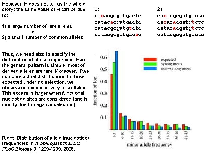
However, H does not tell us the whole story: the same value of H can be due to: 1) a large number of rare alleles or 2) a small number of common alleles Thus, we need also to specify the distribution of allele frequencies. Here the general pattern is simple: most of derived alleles are rare. Moreover, if we compare actual distributions to those expected under no selection, we observe an excess of very rare alleles. This excess is larger when functional nucleotide sites are considered (and is mostly due to negative selection). Right: Distribution of allele (nucleotide) frequencies in Arabidopsis thaliana. PLo. S Biology 3, 1289 -1299, 2005. 1) cacacgcgatgactc catacacgatgactc catacgcgatgtctc catacgcgatgacac 2) cacacgcgatgactc cacacacgatgtctc catacgcgatgactc

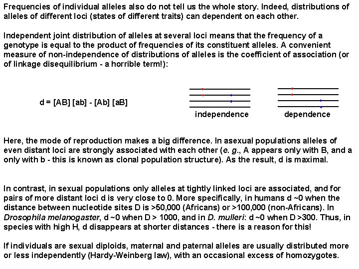
Frequencies of individual alleles also do not tell us the whole story. Indeed, distributions of alleles of different loci (states of different traits) can dependent on each other. Independent joint distribution of alleles at several loci means that the frequency of a genotype is equal to the product of frequencies of its constituent alleles. A convenient measure of non-independence of distributions of alleles is the coefficient of association (or of linkage disequilibrium - a horrible term!): d = [AB] [ab] - [Ab] [a. B] independence dependence Here, the mode of reproduction makes a big difference. In asexual populations alleles of even distant loci are strongly associated with each other (e. g. , A appears only with B, and a only with b - this is known as clonal population structure). As the result, d is maximal. In contrast, in sexual populations only alleles at tightly linked loci are associated, and for pairs of more distant loci d is very close to 0. More specifically, in humans d ~0 when the distance between nucleotide sites D is >50, 000 (Africans) or >100, 000 (non-Africans). In Drosophila melanogaster, d ~0 when D > 1000, and in D. mulleri: d ~0 when D >300. Thus, in species with high H, d disappears at shorter distances - there is a reason for this! If individuals are sexual diploids, maternal and paternal alleles are usually distributed more or less independently (Hardy-Weinberg law), with an occasional excess of homozygotes.

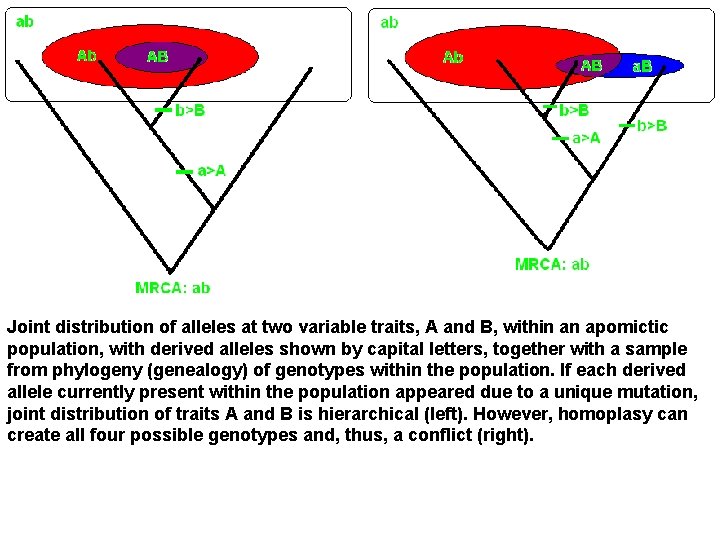
Joint distribution of alleles at two variable traits, A and B, within an apomictic population, with derived alleles shown by capital letters, together with a sample from phylogeny (genealogy) of genotypes within the population. If each derived allele currently present within the population appeared due to a unique mutation, joint distribution of traits A and B is hierarchical (left). However, homoplasy can create all four possible genotypes and, thus, a conflict (right).

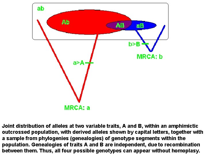
Joint distribution of alleles at two variable traits, A and B, within an amphimictic outcrossed population, with derived alleles shown by capital letters, together with a sample from phylogenies (genealogies) of genotype segments within the population. Genealogies of traits A and B are independent, due to recombination between them. Thus, all four possible genotypes can appear without homoplasy.

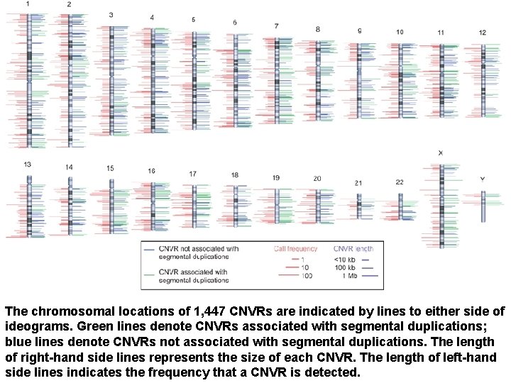
Large-scale genetic differences. Such differences were discovered by Dobzhansky and Sturtevant in 1938, who observed long polymorphic inversions in Drosophila polythene chromosomes using light microscope. Only recently, it became technically possible to study large-scale genetic differences in species without such chromosomes. They turned out to be quite common. A typical human is heterozygous for ~50 deletions larger than 5, 000 nucleotides each, totaling ~750 kb of sequence (Nature Genetics 38, 75 - 81, 2006). A total of 1, 447 copy number variable regions (CNVRs), which can encompass overlapping or adjacent gains or losses, covering 360 megabases (12% of the genome) were identified in 270 humans from four populations with ancestry in Europe, Africa or Asia. These CNVRs contained hundreds of genes, disease loci, functional elements and segmental duplications. Notably, the CNVRs encompassed more nucleotide content per genome than SNPs (Nature 444, 444454, 2006). The excess of rare derived alleles in large-scale variation is even more pronounced than in small-scale variation.

The chromosomal locations of 1, 447 CNVRs are indicated by lines to either side of ideograms. Green lines denote CNVRs associated with segmental duplications; blue lines denote CNVRs not associated with segmental duplications. The length of right-hand side lines represents the size of each CNVR. The length of left-hand side lines indicates the frequency that a CNVR is detected.

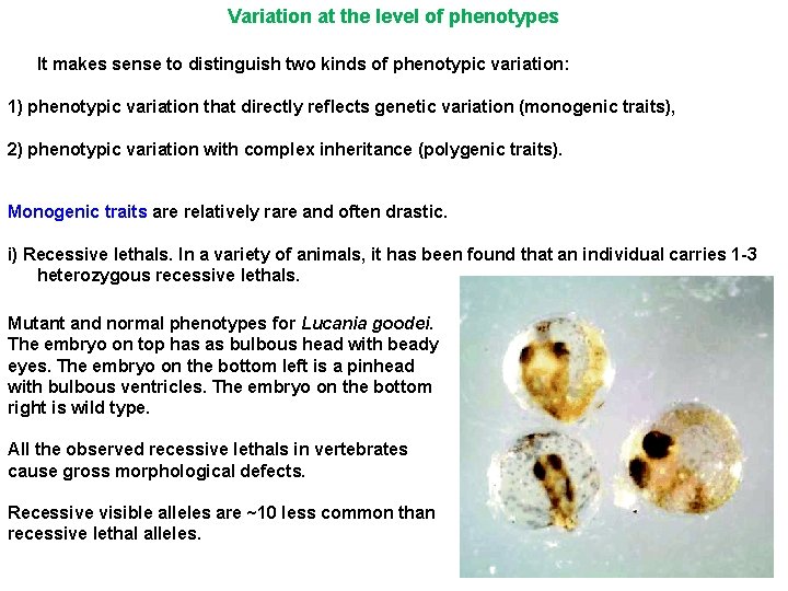
Variation at the level of phenotypes It makes sense to distinguish two kinds of phenotypic variation: 1) phenotypic variation that directly reflects genetic variation (monogenic traits), 2) phenotypic variation with complex inheritance (polygenic traits). Monogenic traits are relatively rare and often drastic. i) Recessive lethals. In a variety of animals, it has been found that an individual carries 1 -3 heterozygous recessive lethals. Mutant and normal phenotypes for Lucania goodei. The embryo on top has as bulbous head with beady eyes. The embryo on the bottom left is a pinhead with bulbous ventricles. The embryo on the bottom right is wild type. All the observed recessive lethals in vertebrates cause gross morphological defects. Recessive visible alleles are ~10 less common than recessive lethal alleles.

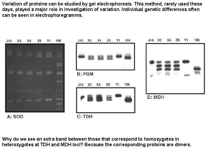
Variation of proteins can be studied by gel electrophoresis. This method, rarely used these days, played a major role in investigation of variation. Individual genetic differences often can be seen in electrophoregramms. Why do we see an extra band between those that correspond to homozygotes in heterozygotes at TDH and MDH loci? Because the corresponding proteins are dimers.

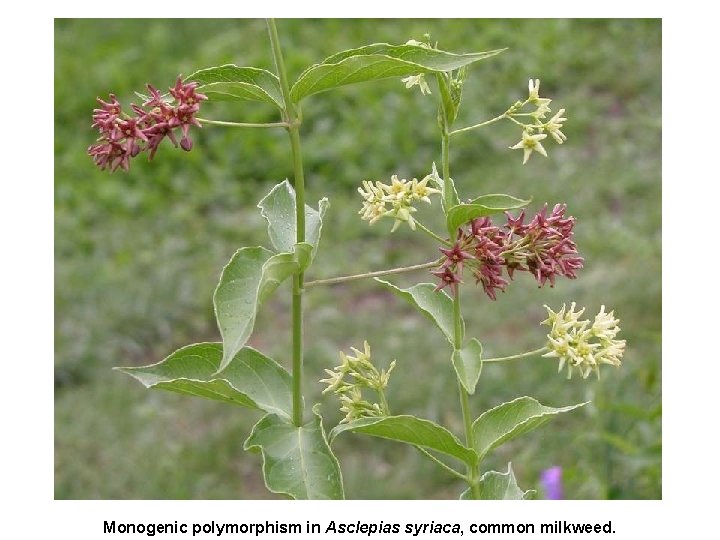
Monogenic polymorphism in Asclepias syriaca, common milkweed.

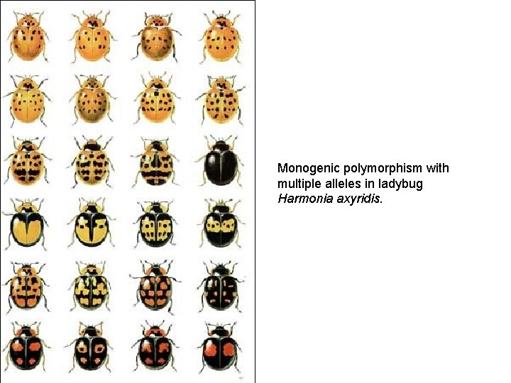
Monogenic polymorphism with multiple alleles in ladybug Harmonia axyridis.

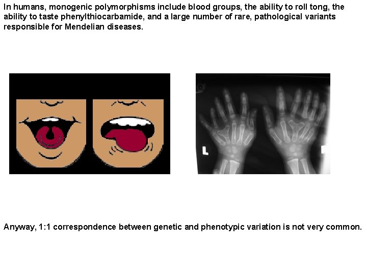
In humans, monogenic polymorphisms include blood groups, the ability to roll tong, the ability to taste phenylthiocarbamide, and a large number of rare, pathological variants responsible for Mendelian diseases. Anyway, 1: 1 correspondence between genetic and phenotypic variation is not very common.

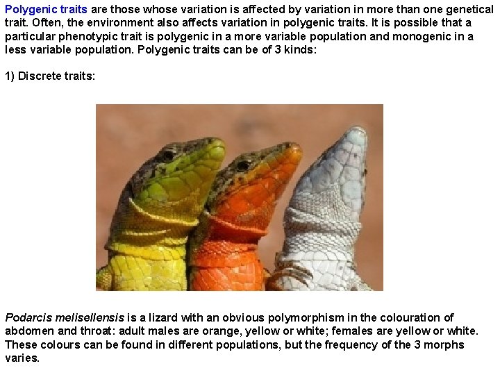
Polygenic traits are those whose variation is affected by variation in more than one genetical trait. Often, the environment also affects variation in polygenic traits. It is possible that a particular phenotypic trait is polygenic in a more variable population and monogenic in a less variable population. Polygenic traits can be of 3 kinds: 1) Discrete traits: Podarcis melisellensis is a lizard with an obvious polymorphism in the colouration of abdomen and throat: adult males are orange, yellow or white; females are yellow or white. These colours can be found in different populations, but the frequency of the 3 morphs varies.

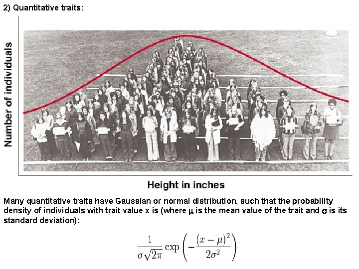
2) Quantitative traits: Many quantitative traits have Gaussian or normal distribution, such that the probability density of individuals with trait value x is (where m is the mean value of the trait and s is its standard deviation):

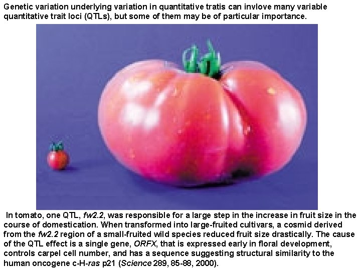
Genetic variation underlying variation in quantitative tratis can invlove many variable quantitative trait loci (QTLs), but some of them may be of particular importance. In tomato, one QTL, fw 2. 2, was responsible for a large step in the increase in fruit size in the course of domestication. When transformed into large-fruited cultivars, a cosmid derived from the fw 2. 2 region of a small-fruited wild species reduced fruit size drastically. The cause of the QTL effect is a single gene, ORFX, that is expressed early in floral development, controls carpel cell number, and has a sequence suggesting structural similarity to the human oncogene c-H-ras p 21 (Science 289, 85 -88, 2000).

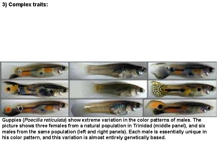
3) Complex traits: Guppies (Poecilia reticulata) show extreme variation in the color patterns of males. The picture shows three females from a natural population in Trinidad (middle panel), and six males from the same population (left and right panels). Each male is essentially unique in his color pattern, and this variation is almost entirely genetically based.

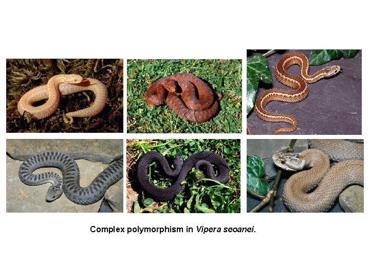
Complex polymorphism in Vipera seoanei.

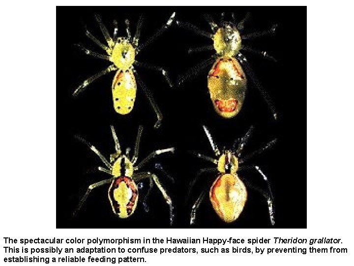
The spectacular color polymorphism in the Hawaiian Happy-face spider Theridon grallator. This is possibly an adaptation to confuse predators, such as birds, by preventing them from establishing a reliable feeding pattern.

Concluding remarks about within-population variation: 1) All populations are variable to some extent, at all levels, 2) Traits and their states responsible for variation come in many different kinds, 3) Genetic variation is ultimately produced by mutation and evaluated by selection, 4) The action of selection upon genetic variation is the key mechanism of Darwinian evolution, and will be treated separately.

Mutation - the first factor of Microevolution Mutation, together with selection, is one of only two factors that are absolutely necessary for Darwinian evolution. What is mutation, mechanistically? - A set of processes that generate mutations, changes of genotypes. There are two such processes: 1) DNA replication, due to errors in it 2) DNA repair, due to errors in it DNA replication struggles to be as precise as physically feasible. The difference between a mutation and a damage must be clearly understood - damages violate integrity of DNA, mutations change its sequence.

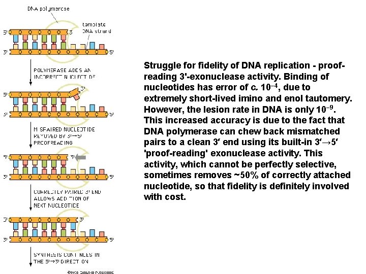
Struggle for fidelity of DNA replication - proofreading 3'-exonuclease activity. Binding of nucleotides has error of c. 10− 4, due to extremely short-lived imino and enol tautomery. However, the lesion rate in DNA is only 10− 9. This increased accuracy is due to the fact that DNA polymerase can chew back mismatched pairs to a clean 3′ end using its built-in 3′→ 5′ 'proof-reading' exonuclease activity. This activity, which cannot be perfectly selective, sometimes removes ~50% of correctly attached nucleotide, so that fidelity is definitely involved with cost.

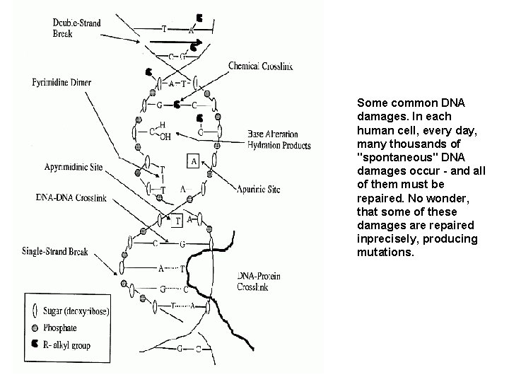
Some common DNA damages. In each human cell, every day, many thousands of "spontaneous" DNA damages occur - and all of them must be repaired. No wonder, that some of these damages are repaired inprecisely, producing mutations.

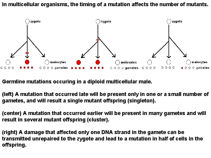
In multicellular organisms, the timing of a mutation affects the number of mutants. Germline mutations occuring in a diploid multicellular male. (left) A mutation that occurred late will be present only in one or a small number of gametes, and will result a single mutant offspring (singleton). (center) A mutation that occurred earlier will be present in many gametes and will result in several mutant offspring (cluster). (right) A damage that affected only one DNA strand in the gamete can be transmitted unrepaired to the zygote and lead to a mutation in half of cells in the offspring.

Why do mutations happen? 1. "Everything consistng of parts crumbles. . . " (Buddha, ~2400 years ago). "Mutations are accidents, and accidents will happen" (Alfred Sturtevant, 1938). 2. Alternatively, mutation can be an adaptation, that enables organisms to occasionally produce improve offspring. To some extent, Buddha and Sturtevant are certainly right: laws of molecular physics do not allow perfect fidelity of DNA handling. If an organism would try to reduce its mutation rate to zero, the cost, in terms of both time and energy, of DNA handling, would approach infinity. We will consider evolution of mutation later.

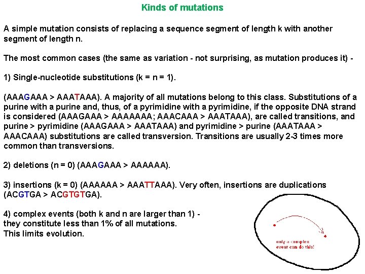
Kinds of mutations A simple mutation consists of replacing a sequence segment of length k with another segment of length n. The most common cases (the same as variation - not surprising, as mutation produces it) - 1) Single-nucleotide substitutions (k = n = 1). (AAAGAAA > AAATAAA). A majority of all mutations belong to this class. Substitutions of a purine with a purine and, thus, of a pyrimidine with a pyrimidine, if the opposite DNA strand is considered (AAAGAAA > AAAAAAA; AAACAAA > AAATAAA), are called transitions, and purine > pyrimidine (AAAGAAA > AAATAAA) and pyrimidine > purine (AAATAAA > AAACAAA) substitutions are called transversion. Transitions are usually 2 -3 times more common than transversions. 2) deletions (n = 0) (AAAGAAA > AAAAAA). 3) insertions (k = 0) (AAAAAA > AAATTAAA). Very often, insertions are duplications (ACGTGA > ACGTGTGA). 4) complex events (both k and n are larger than 1) - they constitute less than 1% of all mutations. This limits evolution.

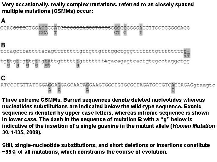
Very occasionally, really complex mutations, referred to as closely spaced multiple mutations (CSMMs) occur: Three extreme CSMMs. Barred sequences denote deleted nucleotides whereas nucleotides substitutions are indicated below the wild-type sequence. Exonic sequence is denoted by upper case letters, whereas intronic sequence is shown in lower case. The dash in the sequence of mutation B with a ‘‘g’’ below is indicative of the insertion of a single guanine in the mutant allele (Human Mutation 30, 1435, 2009). Still, single-nucleotide substitutions, and short deletions or insertions constitute ~99% of all mutations, which constrains the course of evolution.

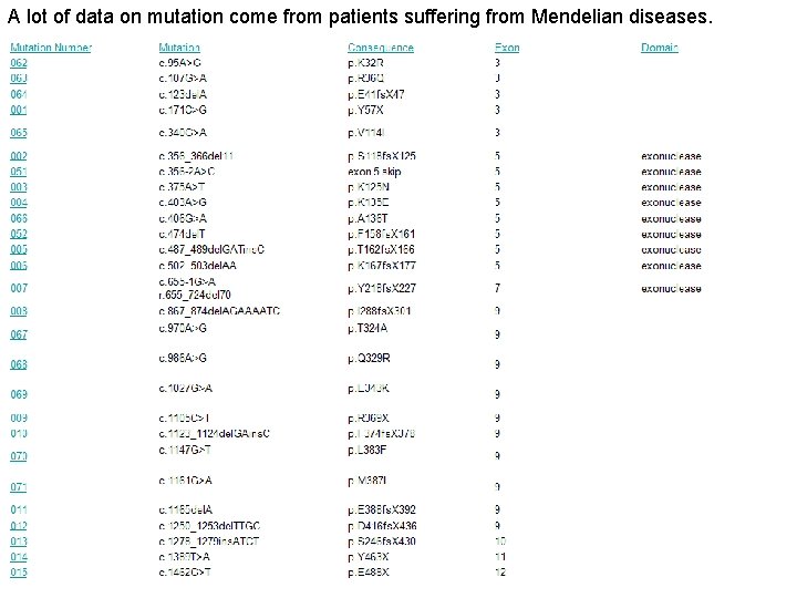
A lot of data on mutation come from patients suffering from Mendelian diseases.

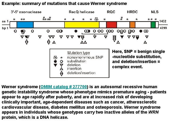
Example: summary of mutations that cause Werner syndrome Here, SNP = benign single -nucleotide substitution, and deletion/insertion = complex event. Werner syndrome (OMIM catalog # 277700) is an autosomal recessive human genetic instability syndrome whose phenotype mimics premature aging - patients appear to age rapidly after puberty, and are at increased risk of developing clinically important, age-dependent diseases such as cancer, atherosclerotic cardiovascular disease, diabetes mellitus and osteoporosis. Werner syndrome appears in individuals whose genotypes carry two inactive alleles of the WRN protein, which is a DNA helicase.

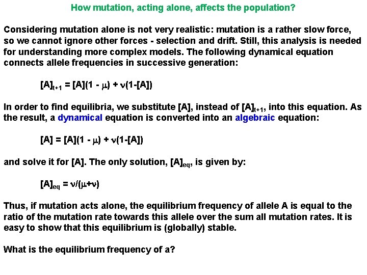
How mutation, acting alone, affects the population? Considering mutation alone is not very realistic: mutation is a rather slow force, so we cannot ignore other forces - selection and drift. Still, this analysis is needed for understanding more complex models. The following dynamical equation connects allele frequencies in successive generation: [A]t+1 = [A](1 - m) + n(1 -[A]) In order to find equilibria, we substitute [A], instead of [A] t+1, into this equation. As the result, a dynamical equation is converted into an algebraic equation: [A] = [A](1 - m) + n(1 -[A]) and solve it for [A]. The only solution, [A]eq, is given by: [A]eq = n/(m+n) Thus, if mutation acts alone, the equilibrium frequency of allele A is equal to the ratio of the mutation rate towards this allele over the sum all mutation rates. It is easy to show that this equilibrium is (globally) stable. What is the equilibrium frequency of a?

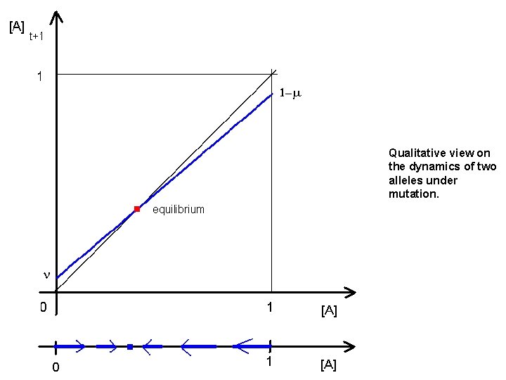
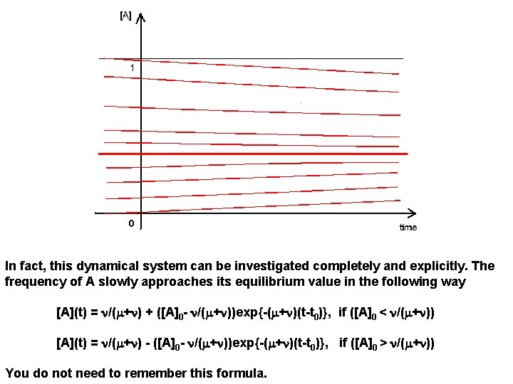
Qualitative view on the dynamics of two alleles under mutation.

In fact, this dynamical system can be investigated completely and explicitly. The frequency of A slowly approaches its equilibrium value in the following way [A](t) = n/(m+n) + ([A]0 - n/(m+n))exp{-(m+n)(t-t 0)}, if ([A]0 < n/(m+n)) [A](t) = n/(m+n) - ([A]0 - n/(m+n))exp{-(m+n)(t-t 0)}, if ([A]0 > n/(m+n)) You do not need to remember this formula.

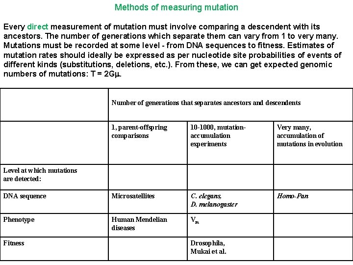
Methods of measuring mutation Every direct measurement of mutation must involve comparing a descendent with its ancestors. The number of generations which separate them can vary from 1 to very many. Mutations must be recorded at some level - from DNA sequences to fitness. Estimates of mutation rates should ideally be expressed as per nucleotide site probabilities of events of different kinds (substitutions, deletions, etc. ). From these, we can get expected genomic numbers of mutations: T = 2 Gm. Number of generations that separates ancestors and descendents 1, parent-offspring comparisons 10 -1000, mutationaccumulation experiments Very many, accumulation of mutations in evolution DNA sequence Microsatellites C. elegans, D. melanogaster Homo-Pan Phenotype Human Mendelian diseases Vm Level at which mutations are detected: Fitness Drosophila, Mukai et al.

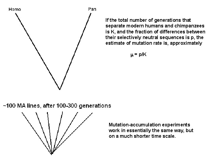
If the total number of generations that separate modern humans and chimpanzees is K, and the fraction of differences between their selectively neutral sequences is p, the estimate of mutation rate is, approximately m = p/K Mutation-accumulation experiments work in essentially the same way, but on a much shorter time scale.

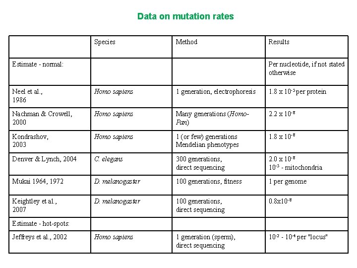
Data on mutation rates Species Method Estimate - normal: Results Per nucleotide, if not stated otherwise Neel et al. , 1986 Homo sapiens 1 generation, electrophoresis 1. 8 x 10 -5 per protein Nachman & Crowell, 2000 Homo sapiens Many generations (Homo. Pan) 2. 2 x 10 -8 Kondrashov, 2003 Homo sapiens 1 (or few) generations Mendelian phenotypes 1. 8 x 10 -8 Denver & Lynch, 2004 C. elegans 300 generations, direct sequencing 2. 0 x 10 -8 10 -5 - mitochondria Mukai 1964, 1972 D. melanogaster 100 generations, fitness 1 per genome Keightley et al. , 2007 D. melanogaster 100 generations, direct sequencing 0. 8 x 10 -8 Homo sapiens 1 generation (sperm), direct sequencing 10 -2 - 10 -4 per "locus" Estimate - hot-spots: Jeffreys et al. , 2002

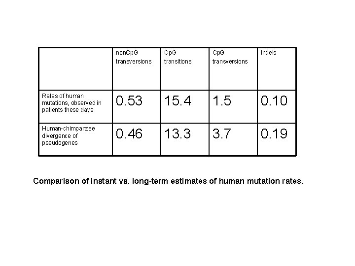
non. Cp. G transversions Cp. G transitions Cp. G transversions indels Rates of human mutations, observed in patients these days 0. 53 15. 4 1. 5 0. 10 Human-chimpanzee divergence of pseudogenes 0. 46 13. 3 3. 7 0. 19 Comparison of instant vs. long-term estimates of human mutation rates.

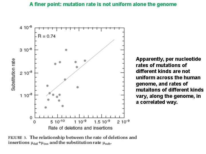
A finer point: mutation rate is not uniform alone the genome Apparently, per nucleotide rates of mutations of different kinds are not uniform across the human genome, and rates of mutaitons of different kinds vary, along the genome, in a correlated way.

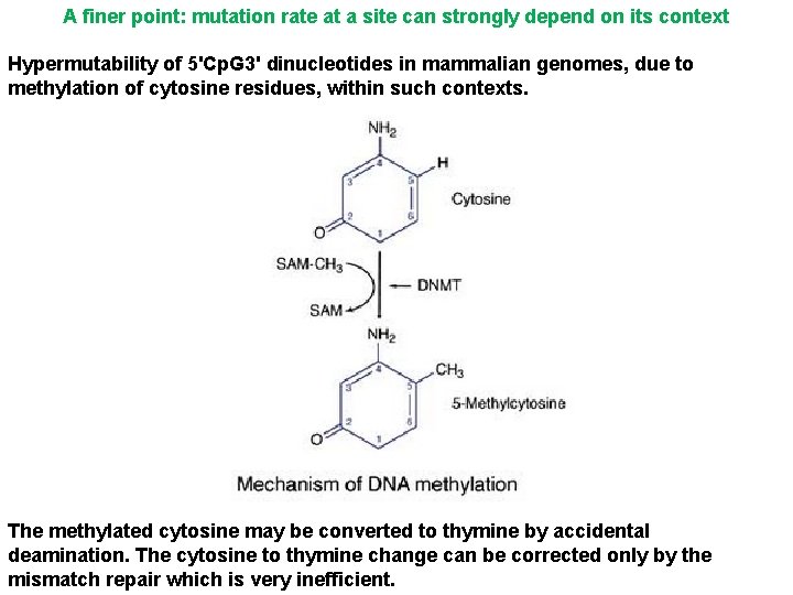
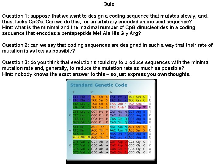
A finer point: mutation rate at a site can strongly depend on its context Hypermutability of 5'Cp. G 3' dinucleotides in mammalian genomes, due to methylation of cytosine residues, within such contexts. The methylated cytosine may be converted to thymine by accidental deamination. The cytosine to thymine change can be corrected only by the mismatch repair which is very inefficient.

As a result, C>T transition rate if ~15 times higher for C's that are within Cp. G contexts, than for C's that are outside Cp. G contexts. Thus, mammalian genomes are strongly depleted of Cp. G dinucleotides - in noncoding DNA, such dinucleotides constitute only ~1% of all dinucleotides, instead of ~6% (1/16) expected. However, coding exons contain a much higher fraction of Cp. G dinucleotides. As a result, a large fraction of human pathogenic missense and nonsense mutations (~40%) occur within Cp. G's, mostly those that encode arginine.

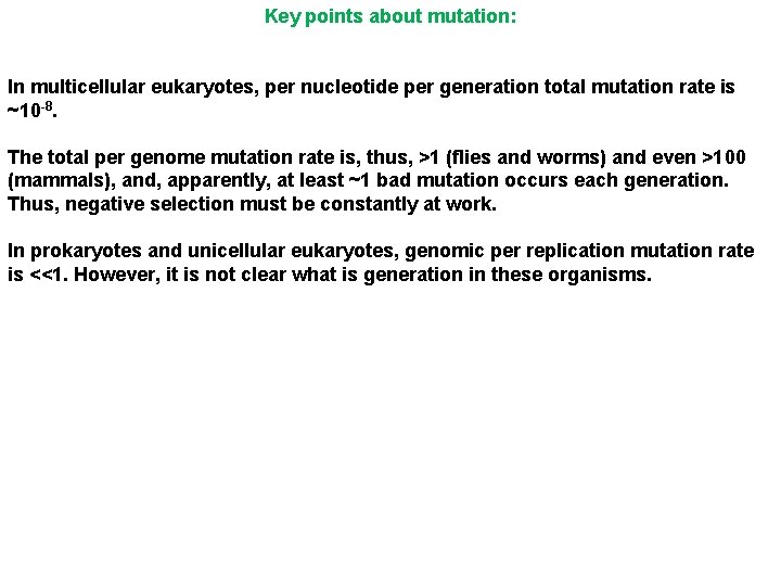
Key points about mutation: In multicellular eukaryotes, per nucleotide per generation total mutation rate is ~10 -8. The total per genome mutation rate is, thus, >1 (flies and worms) and even >100 (mammals), and, apparently, at least ~1 bad mutation occurs each generation. Thus, negative selection must be constantly at work. In prokaryotes and unicellular eukaryotes, genomic per replication mutation rate is <<1. However, it is not clear what is generation in these organisms.

Quiz: Question 1: suppose that we want to design a coding sequence that mutates slowly, and, thus, lacks Cp. G's. Can we do this, for an arbitrary encoded amino acid sequence? Hint: what is the minimal and the maximal number of Cp. G dinucleotides in a coding sequence that encodes a pentapeptide Met Ala His Gly Arg? Question 2: can we say that coding sequences are designed in such a way that their rate of mutation is as low as possible? Question 3: do you think that evolution should try to produce sequences with the minimal mutation rate and, generally, to reduce the mutation rate as much as possible? Hint: nobody knows the exact answer to this – so just express you own thoughts.