Tools for High Performance Scientific Computing Kathy Yelick

Tools for High Performance Scientific Computing Kathy Yelick U. C. Berkeley http: //www. cs. berkeley. edu/~yelick/

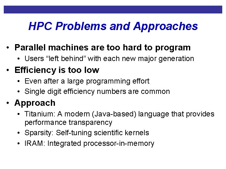
HPC Problems and Approaches • Parallel machines are too hard to program • Users “left behind” with each new major generation • Efficiency is too low • Even after a large programming effort • Single digit efficiency numbers are common • Approach • Titanium: A modern (Java-based) language that provides performance transparency • Sparsity: Self-tuning scientific kernels • IRAM: Integrated processor-in-memory

Titanium: A Global Address Space Language Based on Java • Faculty • • Susan Graham Paul Hilfinger Katherine Yelick Alex Aiken • LBNL collaborators • Phillip Colella • Peter Mc. Quorquodale • Mike Welcome • Students • • • Dan Bonachea Szu-Huey Chang Carrie Fei Ben Liblit Robert Lin Geoff Pike Jimmy Su Ellen Tsai Mike Welcome (LBNL) Siu Man Yau http: //titanium. cs. berkeley. edu/

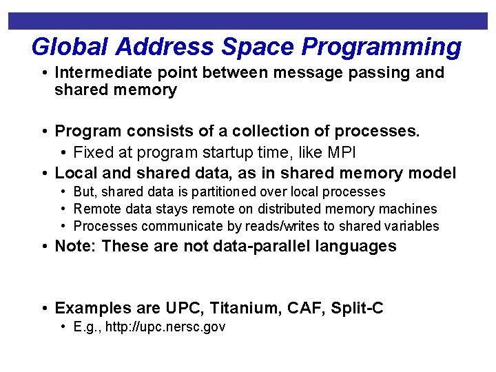
Global Address Space Programming • Intermediate point between message passing and shared memory • Program consists of a collection of processes. • Fixed at program startup time, like MPI • Local and shared data, as in shared memory model • But, shared data is partitioned over local processes • Remote data stays remote on distributed memory machines • Processes communicate by reads/writes to shared variables • Note: These are not data-parallel languages • Examples are UPC, Titanium, CAF, Split-C • E. g. , http: //upc. nersc. gov

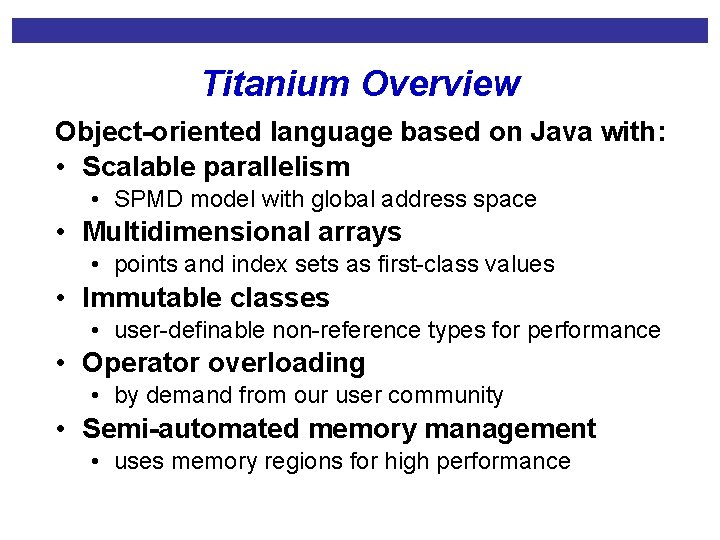
Titanium Overview Object-oriented language based on Java with: • Scalable parallelism • SPMD model with global address space • Multidimensional arrays • points and index sets as first-class values • Immutable classes • user-definable non-reference types for performance • Operator overloading • by demand from our user community • Semi-automated memory management • uses memory regions for high performance

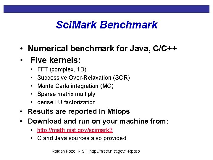
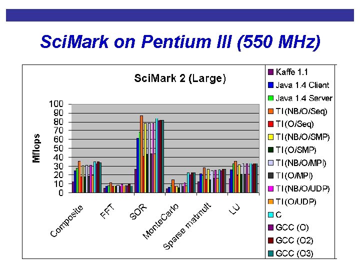
Sci. Mark Benchmark • Numerical benchmark for Java, C/C++ • Five kernels: • • • FFT (complex, 1 D) Successive Over-Relaxation (SOR) Monte Carlo integration (MC) Sparse matrix multiply dense LU factorization • Results are reported in Mflops • Download and run on your machine from: • http: //math. nist. gov/scimark 2 • C and Java sources also provided Roldan Pozo, NIST, http: //math. nist. gov/~Rpozo

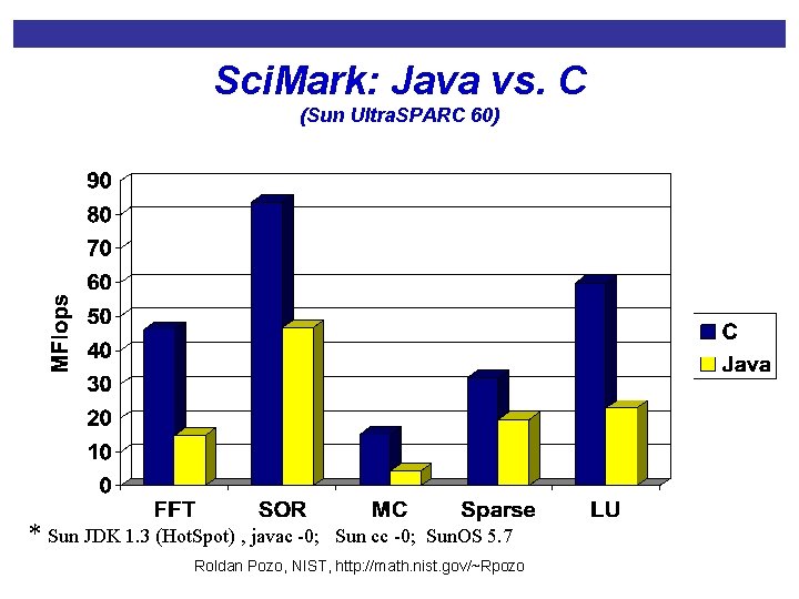
Sci. Mark: Java vs. C (Sun Ultra. SPARC 60) * Sun JDK 1. 3 (Hot. Spot) , javac -0; Sun cc -0; Sun. OS 5. 7 Roldan Pozo, NIST, http: //math. nist. gov/~Rpozo

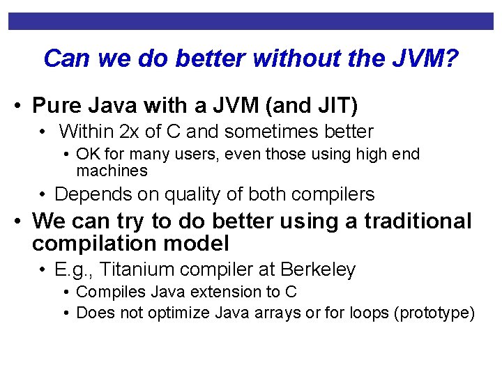
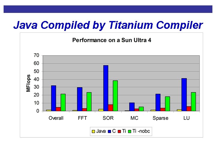
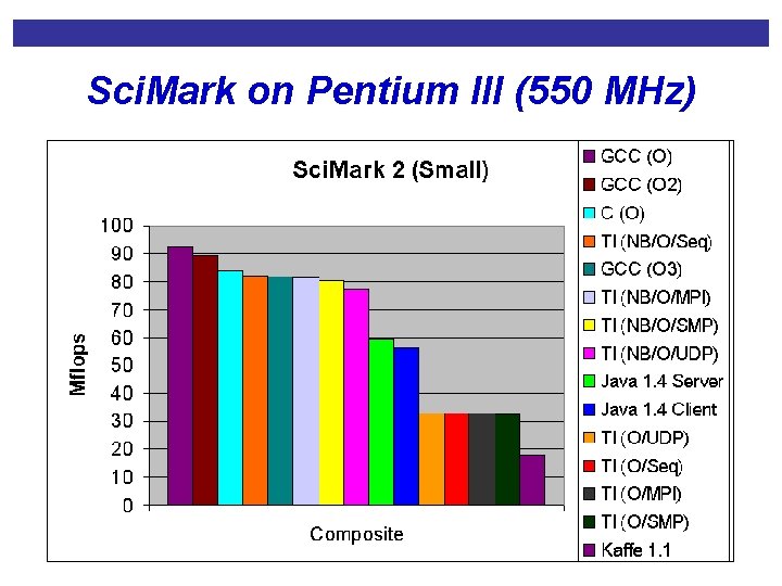
Can we do better without the JVM? • Pure Java with a JVM (and JIT) • Within 2 x of C and sometimes better • OK for many users, even those using high end machines • Depends on quality of both compilers • We can try to do better using a traditional compilation model • E. g. , Titanium compiler at Berkeley • Compiles Java extension to C • Does not optimize Java arrays or for loops (prototype)

Java Compiled by Titanium Compiler

Sci. Mark on Pentium III (550 MHz)

Sci. Mark on Pentium III (550 MHz)

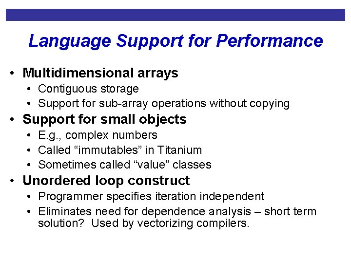
Language Support for Performance • Multidimensional arrays • Contiguous storage • Support for sub-array operations without copying • Support for small objects • E. g. , complex numbers • Called “immutables” in Titanium • Sometimes called “value” classes • Unordered loop construct • Programmer specifies iteration independent • Eliminates need for dependence analysis – short term solution? Used by vectorizing compilers.

Optimizing Parallel Code • Compiler writers would like to move code around • The hardware folks also want to build hardware that dynamically moves operations around • When is reordering correct? • Because the programs are parallel, there are more restrictions, not fewer • The reason is that we have to preserve semantics of what may be viewed by other processors

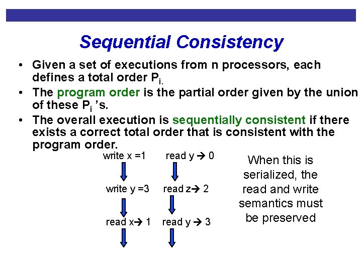
Sequential Consistency • Given a set of executions from n processors, each defines a total order Pi. • The program order is the partial order given by the union of these Pi ’s. • The overall execution is sequentially consistent if there exists a correct total order that is consistent with the program order. write x =1 read y 0 When this is serialized, the write y =3 read z 2 read and write semantics must be preserved read x 1 read y 3

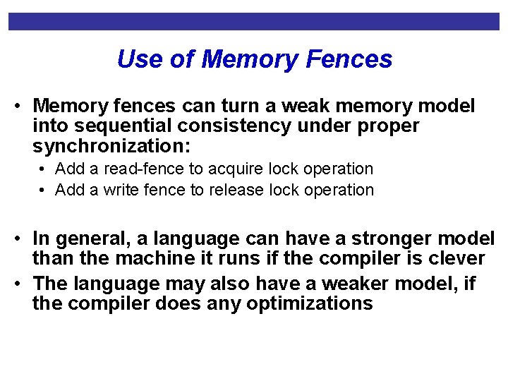
Use of Memory Fences • Memory fences can turn a weak memory model into sequential consistency under proper synchronization: • Add a read-fence to acquire lock operation • Add a write fence to release lock operation • In general, a language can have a stronger model than the machine it runs if the compiler is clever • The language may also have a weaker model, if the compiler does any optimizations

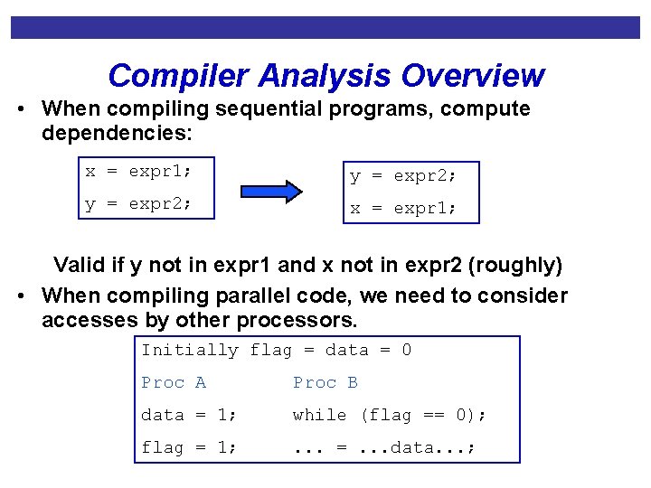
Compiler Analysis Overview • When compiling sequential programs, compute dependencies: x = expr 1; y = expr 2; x = expr 1; Valid if y not in expr 1 and x not in expr 2 (roughly) • When compiling parallel code, we need to consider accesses by other processors. Initially flag = data = 0 Proc A Proc B data = 1; while (flag == 0); flag = 1; . . . =. . . data. . . ;

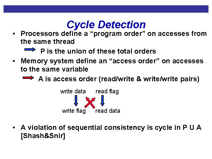
Cycle Detection • Processors define a “program order” on accesses from the same thread P is the union of these total orders • Memory system define an “access order” on accesses to the same variable A is access order (read/write & write/write pairs) write data read flag write flag read data • A violation of sequential consistency is cycle in P U A [Shash&Snir]

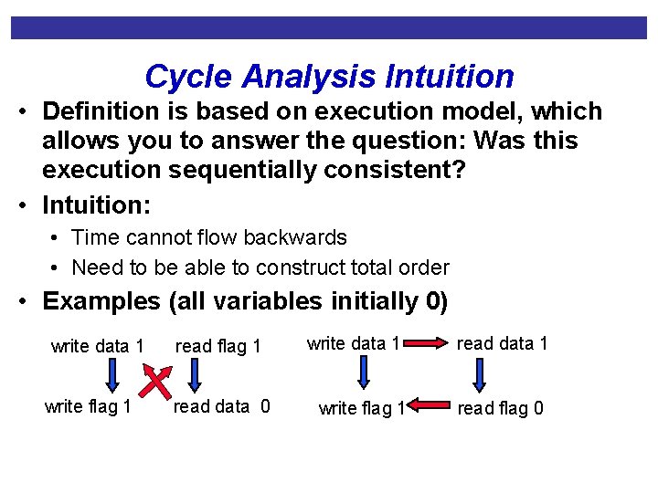
Cycle Analysis Intuition • Definition is based on execution model, which allows you to answer the question: Was this execution sequentially consistent? • Intuition: • Time cannot flow backwards • Need to be able to construct total order • Examples (all variables initially 0) write data 1 write flag 1 read data 0 write data 1 write flag 1 read data 1 read flag 0

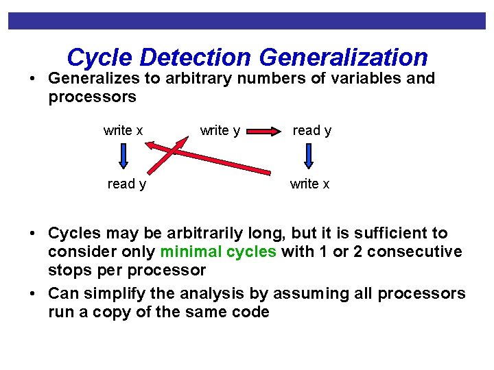
Cycle Detection Generalization • Generalizes to arbitrary numbers of variables and processors write x read y write y read y write x • Cycles may be arbitrarily long, but it is sufficient to consider only minimal cycles with 1 or 2 consecutive stops per processor • Can simplify the analysis by assuming all processors run a copy of the same code

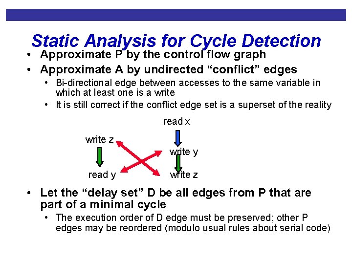
Static Analysis for Cycle Detection • Approximate P by the control flow graph • Approximate A by undirected “conflict” edges • Bi-directional edge between accesses to the same variable in which at least one is a write • It is still correct if the conflict edge set is a superset of the reality read x write z write y read y write z • Let the “delay set” D be all edges from P that are part of a minimal cycle • The execution order of D edge must be preserved; other P edges may be reordered (modulo usual rules about serial code)

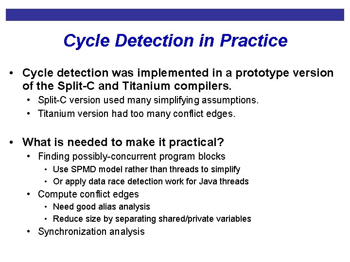
Cycle Detection in Practice • Cycle detection was implemented in a prototype version of the Split-C and Titanium compilers. • Split-C version used many simplifying assumptions. • Titanium version had too many conflict edges. • What is needed to make it practical? • Finding possibly-concurrent program blocks • Use SPMD model rather than threads to simplify • Or apply data race detection work for Java threads • Compute conflict edges • Need good alias analysis • Reduce size by separating shared/private variables • Synchronization analysis

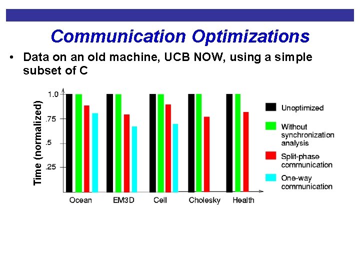
Communication Optimizations Time (normalized) • Data on an old machine, UCB NOW, using a simple subset of C

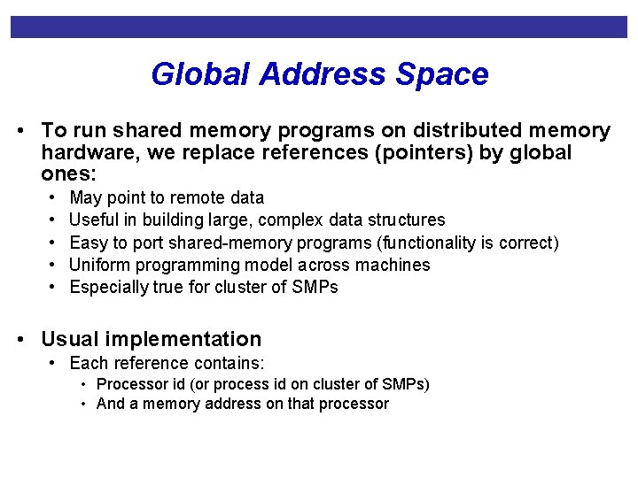
Global Address Space • To run shared memory programs on distributed memory hardware, we replace references (pointers) by global ones: • • • May point to remote data Useful in building large, complex data structures Easy to port shared-memory programs (functionality is correct) Uniform programming model across machines Especially true for cluster of SMPs • Usual implementation • Each reference contains: • Processor id (or process id on cluster of SMPs) • And a memory address on that processor

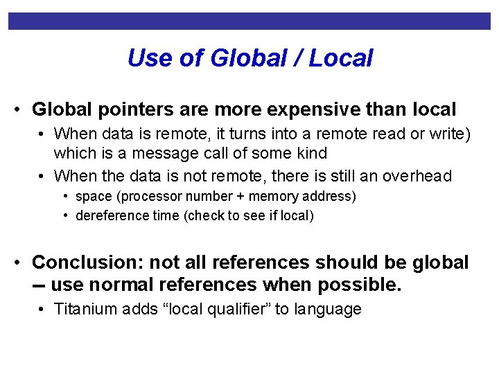
Use of Global / Local • Global pointers are more expensive than local • When data is remote, it turns into a remote read or write) which is a message call of some kind • When the data is not remote, there is still an overhead • space (processor number + memory address) • dereference time (check to see if local) • Conclusion: not all references should be global -- use normal references when possible. • Titanium adds “local qualifier” to language

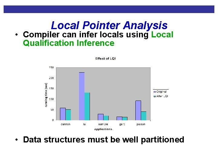
Local Pointer Analysis • Compiler can infer locals using Local Qualification Inference • Data structures must be well partitioned

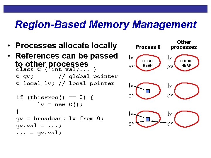
Region-Based Memory Management • Processes allocate locally • References can be passed to other processes class C { int val; . . . } C gv; // global pointer C local lv; // local pointer if (this. Proc() == 0) { lv = new C(); } gv = broadcast lv from 0; gv. val =. . . ; . . . = gv. val; Process 0 lv gv LOCAL HEAP Other processes lv gv lv gv LOCAL HEAP

Parallel Applications • • • Genome Application Heart simulation AMR elliptic and hyperbolic solvers Scalable Poisson for infinite domains Genome application Several smaller benchmarks: EM 3 D, Mat. Mul, LU, FFT, Join,

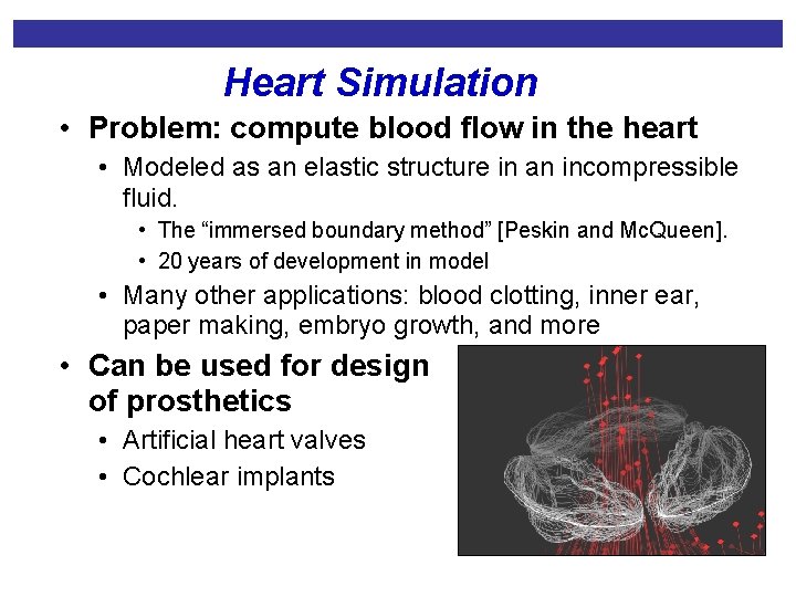
Heart Simulation • Problem: compute blood flow in the heart • Modeled as an elastic structure in an incompressible fluid. • The “immersed boundary method” [Peskin and Mc. Queen]. • 20 years of development in model • Many other applications: blood clotting, inner ear, paper making, embryo growth, and more • Can be used for design of prosthetics • Artificial heart valves • Cochlear implants

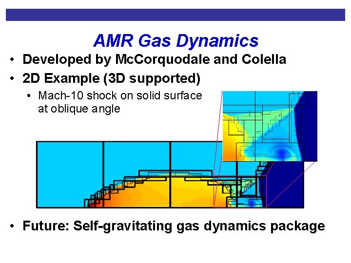
AMR Gas Dynamics • Developed by Mc. Corquodale and Colella • 2 D Example (3 D supported) • Mach-10 shock on solid surface at oblique angle • Future: Self-gravitating gas dynamics package

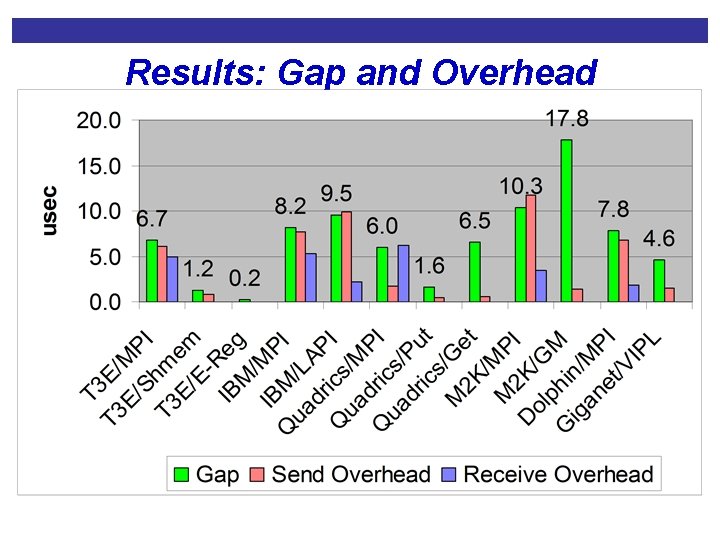
Benchmarks for GAS Languages • EEL – End to end latency or time spent sending a short message between two processes. • BW – Large message network bandwidth • Parameters of the Log. P Model • L – “Latency”or time spent on the network • During this time, processor can be doing other work • O – “Overhead” or processor busy time on the sending or receiving side. • During this time, processor cannot be doing other work • We distinguish between “send” and “recv” overhead • G – “gap” the rate at which messages can be pushed onto the network. • P – the number of processors • This work was done with the UPC group at LBL

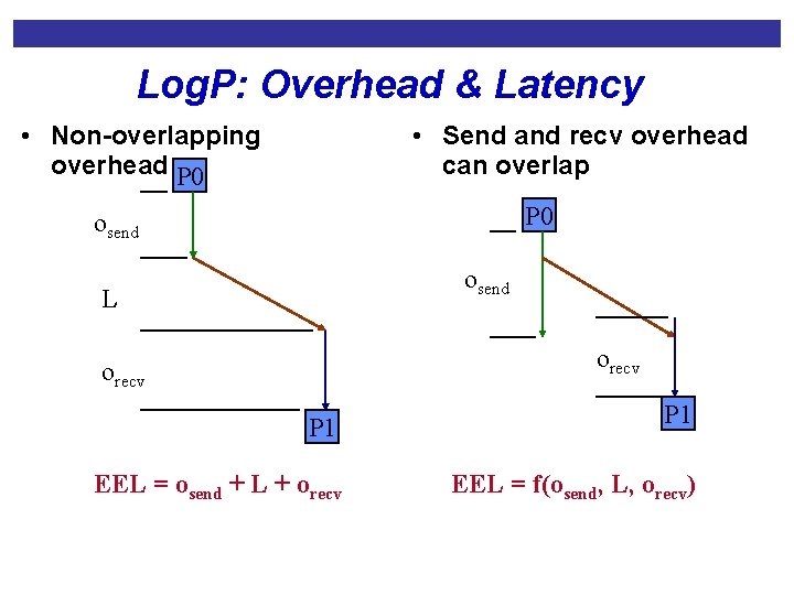
Log. P: Overhead & Latency • Non-overlapping overhead P 0 • Send and recv overhead can overlap P 0 osend L orecv P 1 EEL = osend + L + orecv EEL = f(osend, L, orecv)

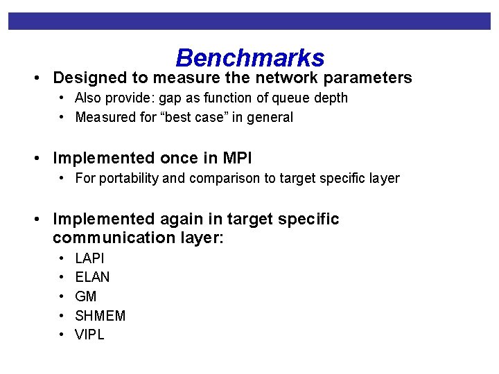
Benchmarks • Designed to measure the network parameters • Also provide: gap as function of queue depth • Measured for “best case” in general • Implemented once in MPI • For portability and comparison to target specific layer • Implemented again in target specific communication layer: • • • LAPI ELAN GM SHMEM VIPL

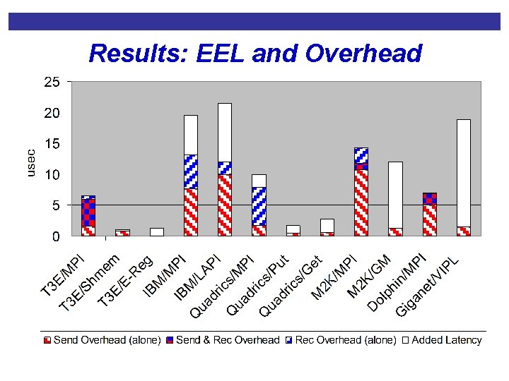
Results: EEL and Overhead

Results: Gap and Overhead

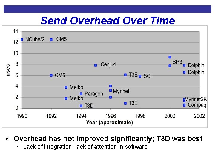
Send Overhead Over Time • Overhead has not improved significantly; T 3 D was best • Lack of integration; lack of attention in software

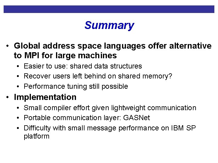
Summary • Global address space languages offer alternative to MPI for large machines • Easier to use: shared data structures • Recover users left behind on shared memory? • Performance tuning still possible • Implementation • Small compiler effort given lightweight communication • Portable communication layer: GASNet • Difficulty with small message performance on IBM SP platform

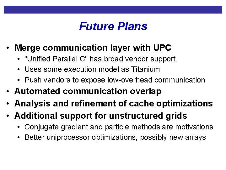
Future Plans • Merge communication layer with UPC • “Unified Parallel C” has broad vendor support. • Uses some execution model as Titanium • Push vendors to expose low-overhead communication • Automated communication overlap • Analysis and refinement of cache optimizations • Additional support for unstructured grids • Conjugate gradient and particle methods are motivations • Better uniprocessor optimizations, possibly new arrays

Sparsity: Self-Tuning Scientific Kernels Faculty James Demmel Katherine Yelick Graduate Students Rich Vuduc Eun-Jim Im • Undergraduates • • • Shoaib Kamil Rajesh Nishtala Benjamin Lee Hyun-Jin Moon Atilla Gyulassy Tuyet-Linh Phan http: //www. cs. berkeley. edu/~yelick/sparsity

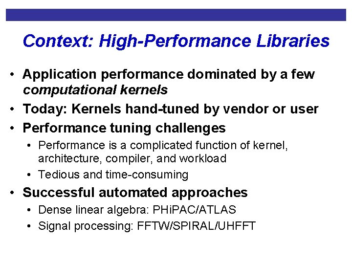
Context: High-Performance Libraries • Application performance dominated by a few computational kernels • Today: Kernels hand-tuned by vendor or user • Performance tuning challenges • Performance is a complicated function of kernel, architecture, compiler, and workload • Tedious and time-consuming • Successful automated approaches • Dense linear algebra: PHi. PAC/ATLAS • Signal processing: FFTW/SPIRAL/UHFFT

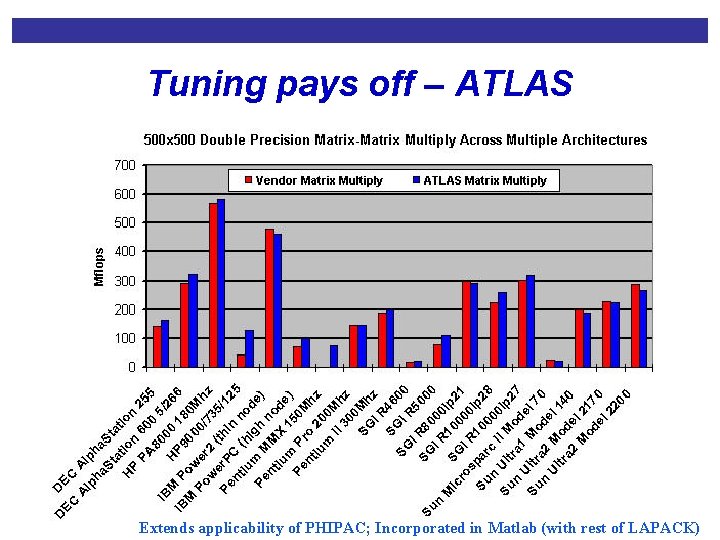
Tuning pays off – ATLAS Extends applicability of PHIPAC; Incorporated in Matlab (with rest of LAPACK)

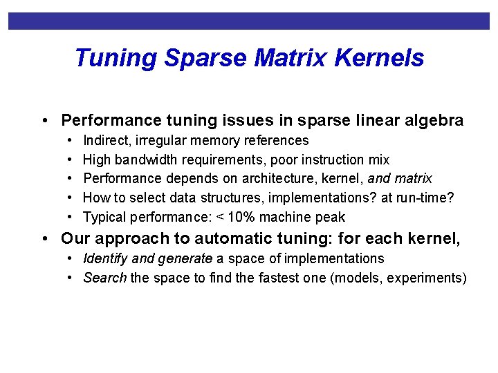
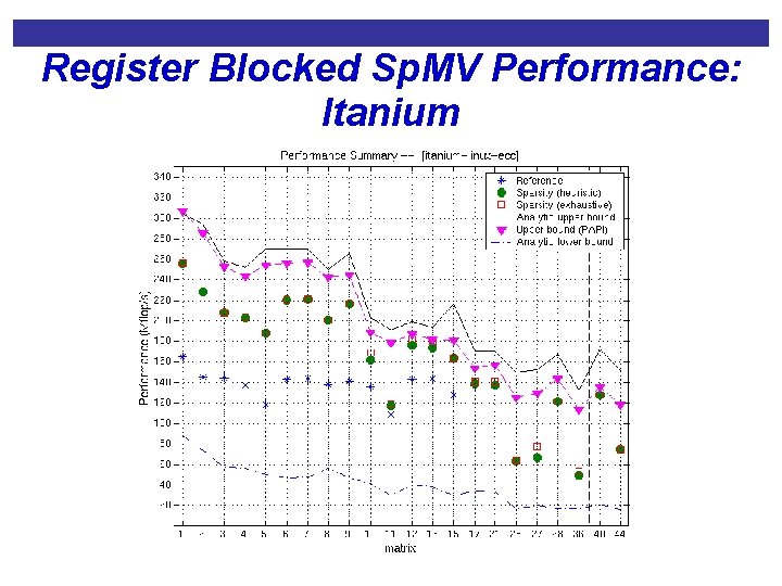
Tuning Sparse Matrix Kernels • Performance tuning issues in sparse linear algebra • • • Indirect, irregular memory references High bandwidth requirements, poor instruction mix Performance depends on architecture, kernel, and matrix How to select data structures, implementations? at run-time? Typical performance: < 10% machine peak • Our approach to automatic tuning: for each kernel, • Identify and generate a space of implementations • Search the space to find the fastest one (models, experiments)

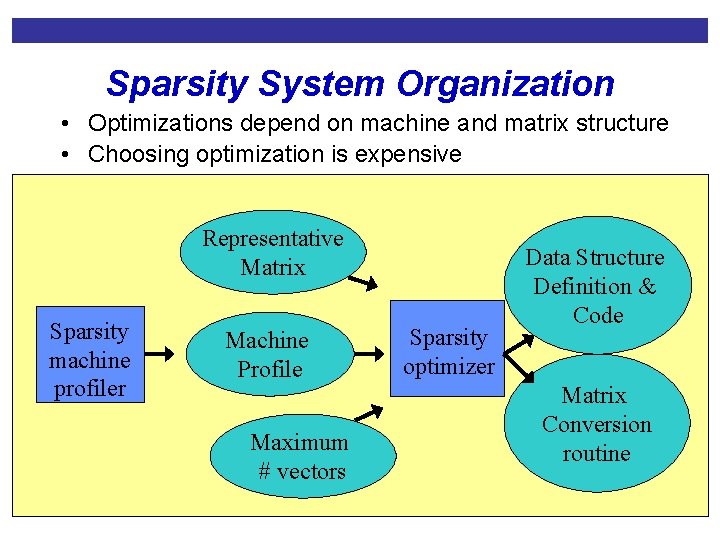
Sparsity System Organization • Optimizations depend on machine and matrix structure • Choosing optimization is expensive Representative Matrix Sparsity machine profiler Machine Profile Maximum # vectors Sparsity optimizer Data Structure Definition & Code Matrix Conversion routine

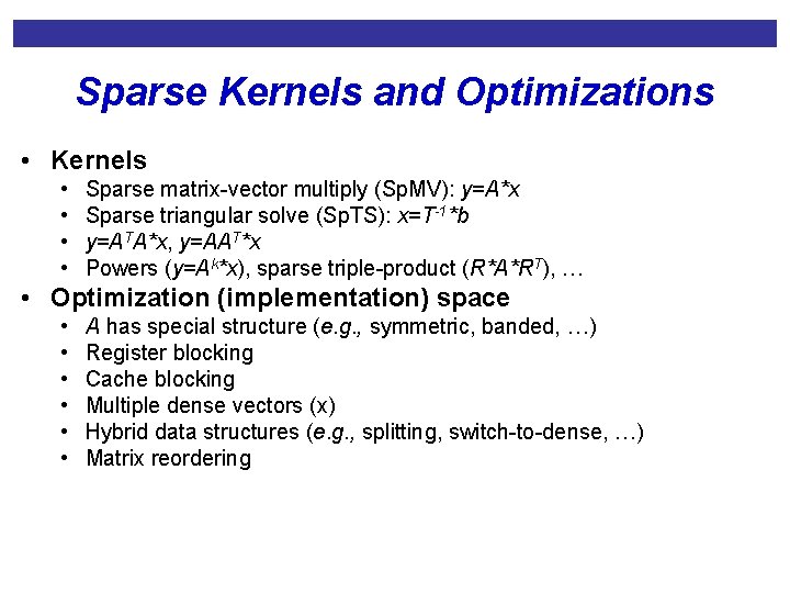
Sparse Kernels and Optimizations • Kernels • • Sparse matrix-vector multiply (Sp. MV): y=A*x Sparse triangular solve (Sp. TS): x=T-1*b y=ATA*x, y=AAT*x Powers (y=Ak*x), sparse triple-product (R*A*RT), … • Optimization (implementation) space • • • A has special structure (e. g. , symmetric, banded, …) Register blocking Cache blocking Multiple dense vectors (x) Hybrid data structures (e. g. , splitting, switch-to-dense, …) Matrix reordering

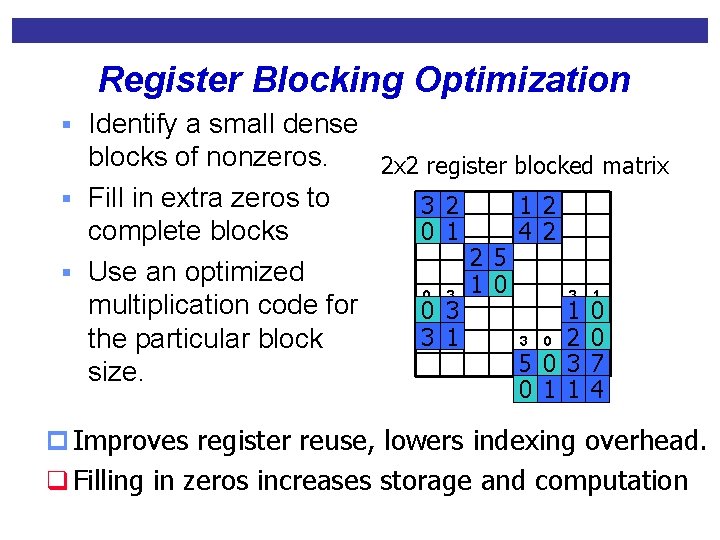
Register Blocking Optimization § Identify a small dense blocks of nonzeros. 2 x 2 register blocked matrix § Fill in extra zeros to 32 21 14 23 00 12 41 22 complete blocks 1 2 21 50 § Use an optimized 1 0 0 3 3 1 multiplication code for 02 35 11 04 3 1 3 0 2 the particular block 50 04 31 72 size. 0 1 1 4 p Improves register reuse, lowers indexing overhead. q Filling in zeros increases storage and computation

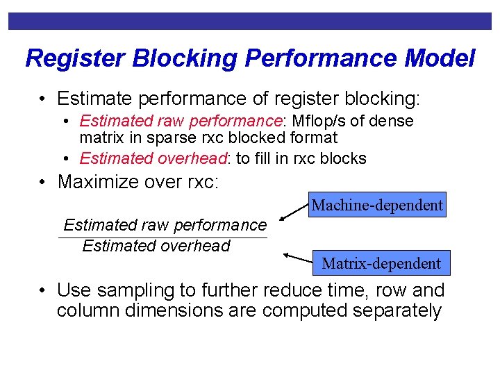
Register Blocking Performance Model • Estimate performance of register blocking: • Estimated raw performance: Mflop/s of dense matrix in sparse rxc blocked format • Estimated overhead: to fill in rxc blocks • Maximize over rxc: Machine-dependent Estimated raw performance Estimated overhead Matrix-dependent • Use sampling to further reduce time, row and column dimensions are computed separately

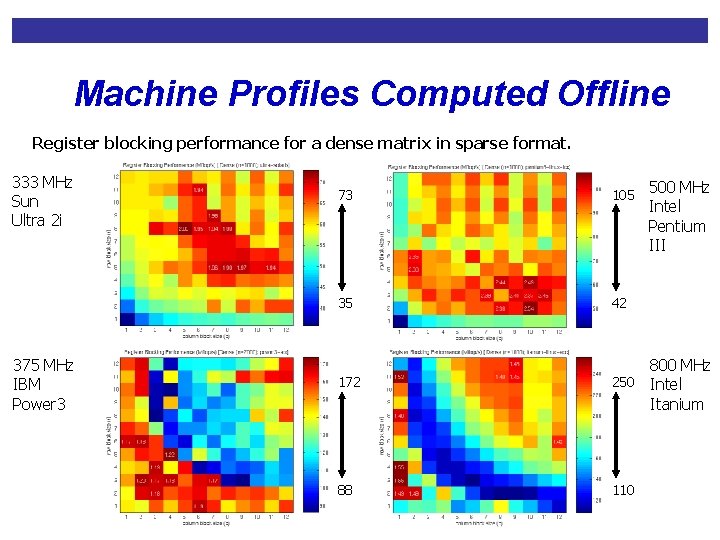
Machine Profiles Computed Offline Register blocking performance for a dense matrix in sparse format. 333 MHz Sun Ultra 2 i 375 MHz IBM Power 3 500 MHz Intel Pentium III 73 105 35 42 172 800 MHz 250 Intel Itanium 88 110

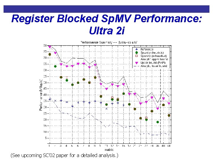
Register Blocked Sp. MV Performance: Ultra 2 i (See upcoming SC’ 02 paper for a detailed analysis. )

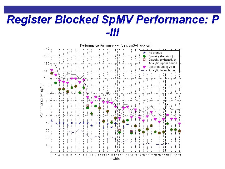
Register Blocked Sp. MV Performance: P -III

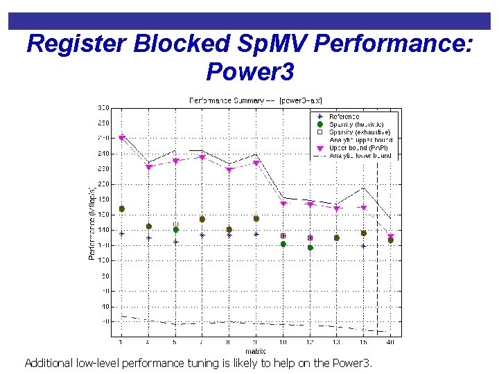
Register Blocked Sp. MV Performance: Power 3 Additional low-level performance tuning is likely to help on the Power 3.

Register Blocked Sp. MV Performance: Itanium

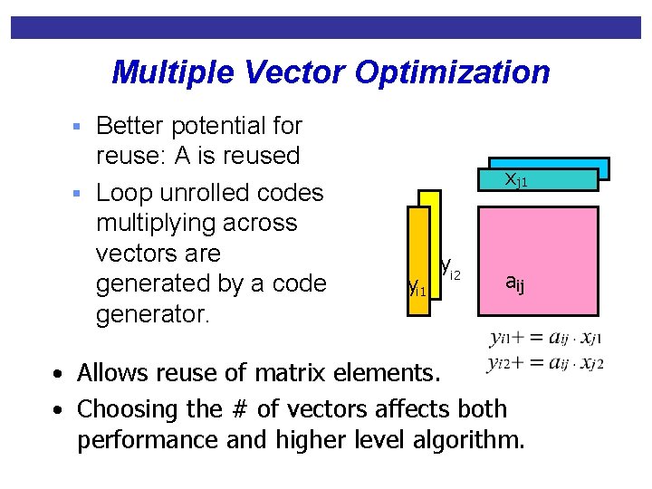
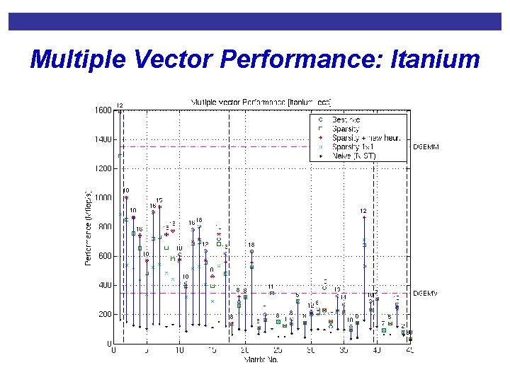
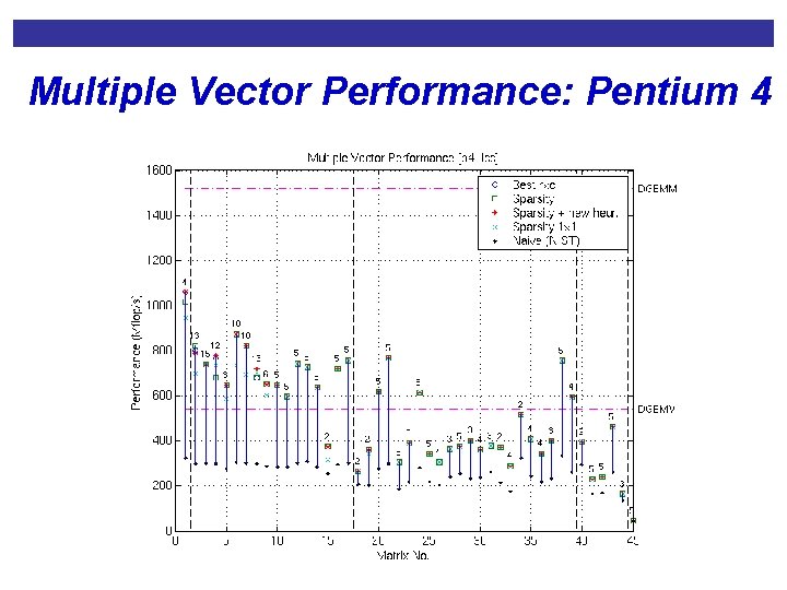
Multiple Vector Optimization § Better potential for reuse: A is reused § Loop unrolled codes multiplying across vectors are generated by a code generator. x j 1 yi 2 aij • Allows reuse of matrix elements. • Choosing the # of vectors affects both performance and higher level algorithm.

Multiple Vector Performance: Itanium

Multiple Vector Performance: Pentium 4

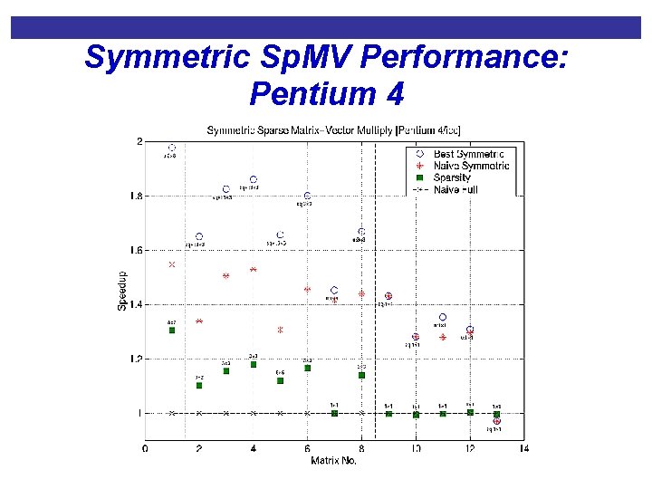
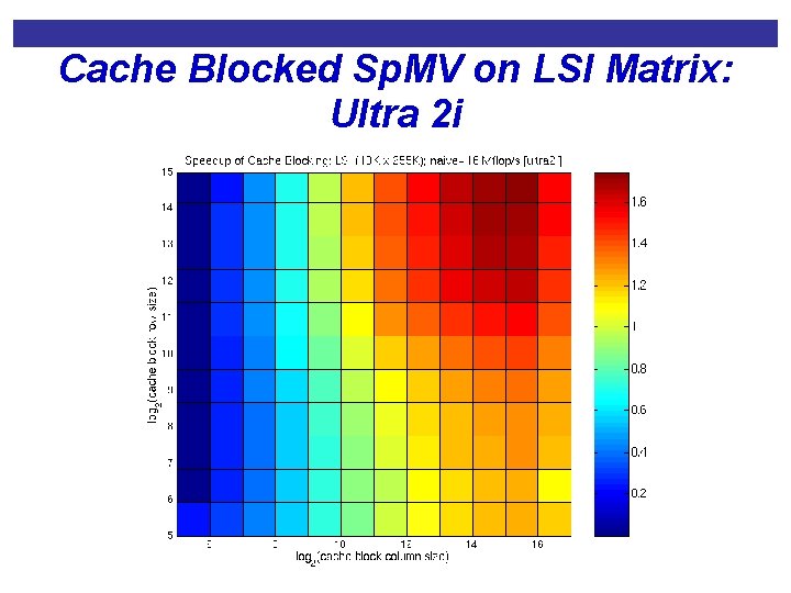
Exploiting Additional Matrix Structure • Symmetry (numerical or structural) • Reuse matrix entries • Can combine with register blocking, multiple vectors, … • Large matrices with random structure • E. g. , Latent Semantic Indexing (LSI) matrices • Technique: cache blocking • Store matrix as 2 i x 2 j sparse submatrices • Useful when source vector is large • Currently, search to find fastest size

Symmetric Sp. MV Performance: Pentium 4

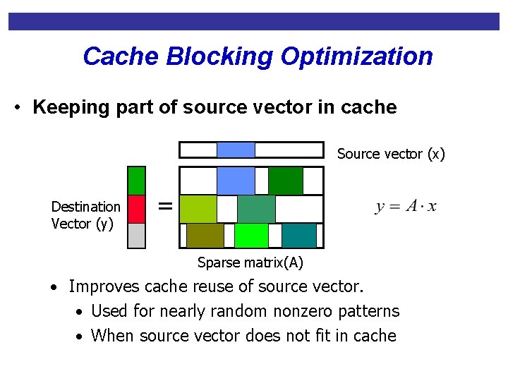
Cache Blocking Optimization • Keeping part of source vector in cache Source vector (x) Destination Vector (y) = Sparse matrix(A) • Improves cache reuse of source vector. • Used for nearly random nonzero patterns • When source vector does not fit in cache

Cache Blocked Sp. MV on LSI Matrix: Ultra 2 i

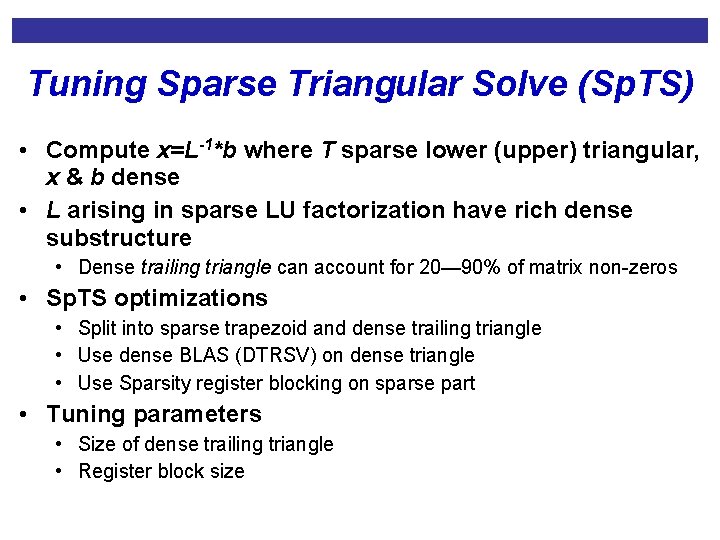
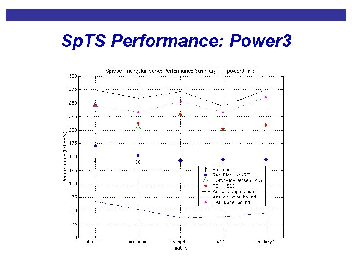
Tuning Sparse Triangular Solve (Sp. TS) • Compute x=L-1*b where T sparse lower (upper) triangular, x & b dense • L arising in sparse LU factorization have rich dense substructure • Dense trailing triangle can account for 20— 90% of matrix non-zeros • Sp. TS optimizations • Split into sparse trapezoid and dense trailing triangle • Use dense BLAS (DTRSV) on dense triangle • Use Sparsity register blocking on sparse part • Tuning parameters • Size of dense trailing triangle • Register block size

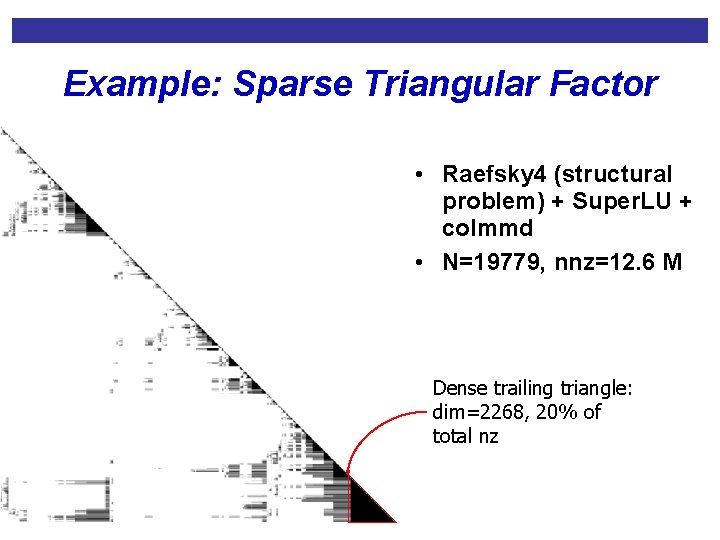
Example: Sparse Triangular Factor • Raefsky 4 (structural problem) + Super. LU + colmmd • N=19779, nnz=12. 6 M Dense trailing triangle: dim=2268, 20% of total nz

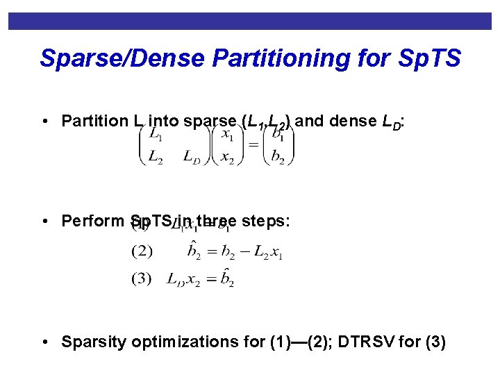
Sparse/Dense Partitioning for Sp. TS • Partition L into sparse (L 1, L 2) and dense LD: • Perform Sp. TS in three steps: • Sparsity optimizations for (1)—(2); DTRSV for (3)

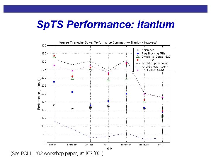
Sp. TS Performance: Itanium (See POHLL ’ 02 workshop paper, at ICS ’ 02. )

Sp. TS Performance: Power 3

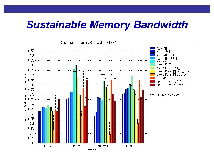
Sustainable Memory Bandwidth

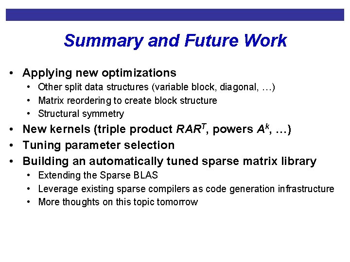
Summary and Future Work • Applying new optimizations • Other split data structures (variable block, diagonal, …) • Matrix reordering to create block structure • Structural symmetry • New kernels (triple product RART, powers Ak, …) • Tuning parameter selection • Building an automatically tuned sparse matrix library • Extending the Sparse BLAS • Leverage existing sparse compilers as code generation infrastructure • More thoughts on this topic tomorrow

IRAM: Intelligent RAM • Faculty • Dave Patterson • Katherine Yelick • Graduate Students • • • Christoforos Kozyrakis Joe Gebis Sam Williams Manikandan Narayanan Iakovos Kosmidakis Iaonnis Kosmidakis • LBNL Collaborators (Benchmarking) • • Parry Husbands Brain Gaeke Xiaoye Li Leonid Oliker • Staff • Dave Judd • Steve Pope

Motivation • Observation: Current cache-based supercomputers perform at a small fraction of peak for memory intensive problems (particularly irregular ones) • E. g. Optimized Sparse Matrix-Vector Multiplication runs at ~ 20% of floating point peak on 1. 5 GHz P 4 • Even worse when parallel efficiency considered • Overall <10% efficiency is typical for many applications • Performance directly related to memory system design • But “gap” between processor performance and DRAM access times continues to grow (60%/yr vs. 7%/yr) • Is memory bandwidth the problem?

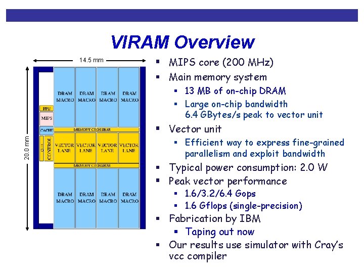
VIRAM Overview 14. 5 mm § MIPS core (200 MHz) § Main memory system § 13 MB of on-chip DRAM § Large on-chip bandwidth 6. 4 GBytes/s peak to vector unit 20. 0 mm § Vector unit § Efficient way to express fine-grained parallelism and exploit bandwidth § Typical power consumption: 2. 0 W § Peak vector performance § 1. 6/3. 2/6. 4 Gops § 1. 6 Gflops (single-precision) § Fabrication by IBM § Taping out now § Our results use simulator with Cray’s vcc compiler

Our Task • Evaluate use of processor-in-memory (PIM) chips as a building block for high performance machines • For now focus on serial performance • Benchmark VIRAM on Scientific Computing kernels • Originally for multimedia applications • Can we use on-chip DRAM for vector processing vs. the conventional SRAM? (DRAM denser) • Isolate performance limiting features of architectures • More than just memory bandwidth

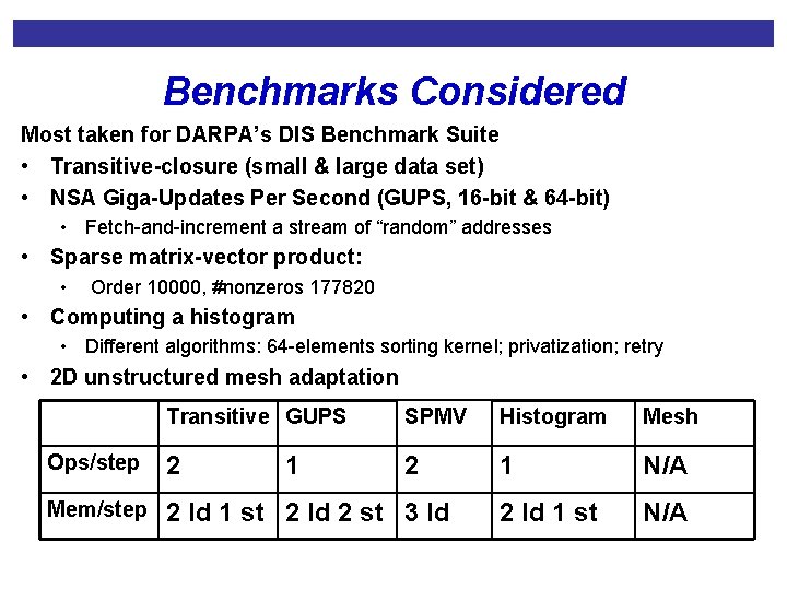
Benchmarks Considered Most taken for DARPA’s DIS Benchmark Suite • Transitive-closure (small & large data set) • NSA Giga-Updates Per Second (GUPS, 16 -bit & 64 -bit) • Fetch-and-increment a stream of “random” addresses • Sparse matrix-vector product: • Order 10000, #nonzeros 177820 • Computing a histogram • Different algorithms: 64 -elements sorting kernel; privatization; retry • 2 D unstructured mesh adaptation Transitive GUPS SPMV Histogram Mesh Ops/step 2 2 1 N/A Mem/step 2 ld 1 st 2 ld 2 st 3 ld 2 ld 1 st N/A 1

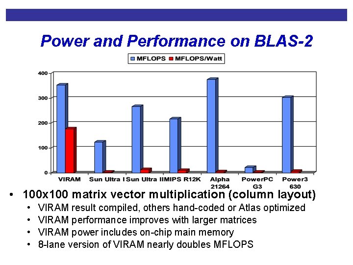
Power and Performance on BLAS-2 • 100 x 100 matrix vector multiplication (column layout) • • VIRAM result compiled, others hand-coded or Atlas optimized VIRAM performance improves with larger matrices VIRAM power includes on-chip main memory 8 -lane version of VIRAM nearly doubles MFLOPS

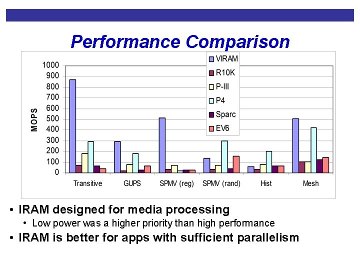
Performance Comparison • IRAM designed for media processing • Low power was a higher priority than high performance • IRAM is better for apps with sufficient parallelism

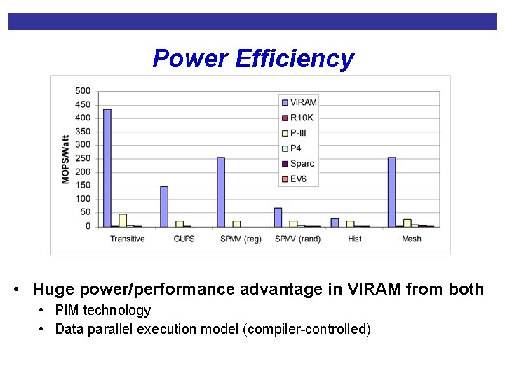
Power Efficiency • Huge power/performance advantage in VIRAM from both • PIM technology • Data parallel execution model (compiler-controlled)

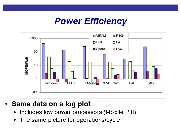
Power Efficiency • Same data on a log plot • Includes low power processors (Mobile PIII) • The same picture for operations/cycle

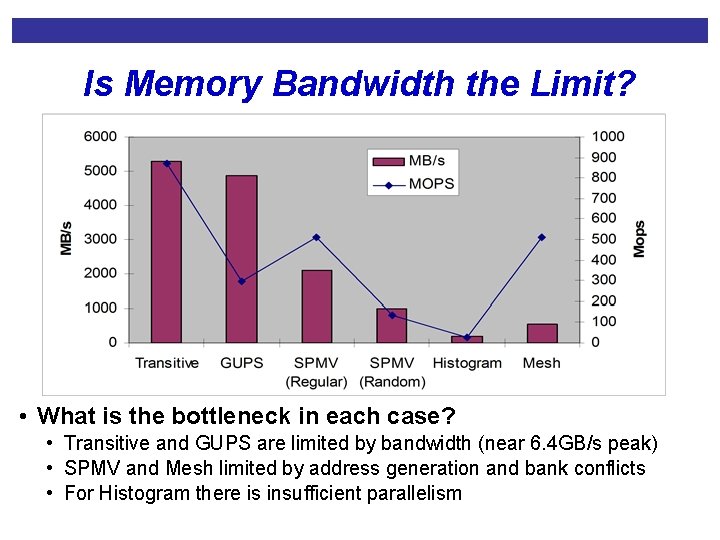
Is Memory Bandwidth the Limit? • What is the bottleneck in each case? • Transitive and GUPS are limited by bandwidth (near 6. 4 GB/s peak) • SPMV and Mesh limited by address generation and bank conflicts • For Histogram there is insufficient parallelism

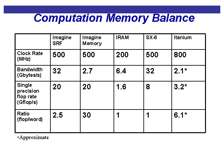
Computation Memory Balance Imagine SRF Imagine Memory IRAM SX-6 Itanium Clock Rate (MHz) 500 200 500 800 Bandwidth (Gbytes/s) 32 2. 7 6. 4 32 2. 1* Single precision flop rate (Gflop/s) 20 20 1. 6 8 3. 2* Ratio (flop/word) 2. 5 30 1 1 6. 1* • Approximate

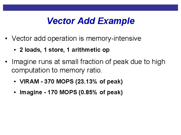
Vector Add Example • Vector add operation is memory-intensive • 2 loads, 1 store, 1 arithmetic op • Imagine runs at small fraction of peak due to high computation to memory ratio. • VIRAM - 370 MOPS (23. 13% of peak) • Imagine - 170 MOPS (0. 85% of peak)

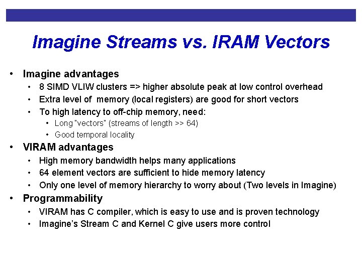
Imagine Streams vs. IRAM Vectors • Imagine advantages • 8 SIMD VLIW clusters => higher absolute peak at low control overhead • Extra level of memory (local registers) are good for short vectors • To high latency to off-chip memory, need: • Long “vectors” (streams of length >> 64) • Good temporal locality • VIRAM advantages • High memory bandwidth helps many applications • 64 element vectors are sufficient to hide memory latency • Only one level of memory hierarchy to worry about (Two levels in Imagine) • Programmability • VIRAM has C compiler, which is easy to use and is proven technology • Imagine’s Stream C and Kernel C give users more control

Summary • Both IRAM and Imagine depend on parallelism • Programmability advantage to VIRAM • All benchmarks vectorized by the VIRAM compiler (Cray vectorizer) • With restructuring and hints from programmers • Performance advantage of VIRAM • Large on applications limited only by bandwidth • More address generators/sub-banks would help irregular performance • Performance/Power advantage of VIRAM • Over both low power and high performance processors • Both PIM and data parallelism are key • Imagine results preliminary • Great peak performance for programs with good temporal locality