tom h wilsongeo wvu edu Department of Geology

tom. h. wilson@geo. wvu. edu Department of Geology and Geography West Virginia University Morgantown, WV

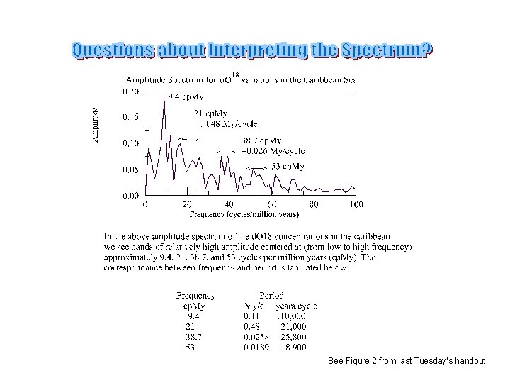
See Figure 2 from last Tuesday’s handout

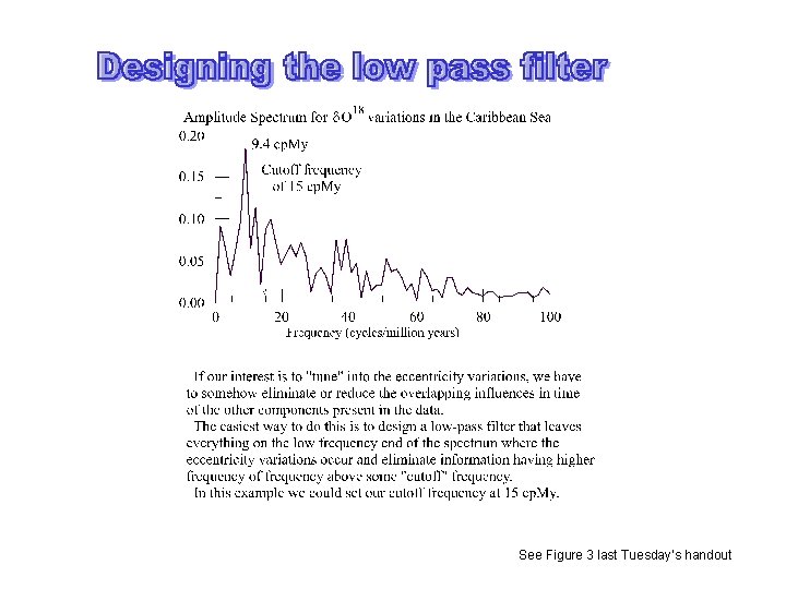
See Figure 3 last Tuesday’s handout

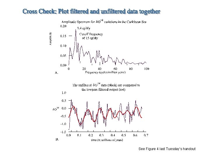
See Figure 4 last Tuesday’s handout

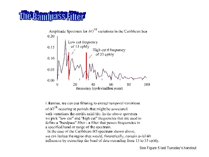
See Figure 5 last Tuesday’s handout

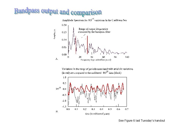
See Figure 6 last Tuesday’s handout

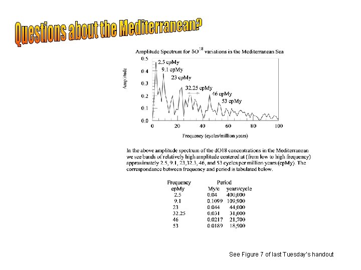
See Figure 7 of last Tuesday’s handout

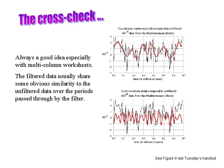
Always a good idea especially with multi-column worksheets. The filtered data usually share some obvious similarity to the unfiltered data over the periods passed through by the filter. See Figure 9 last Tuesday’s handout

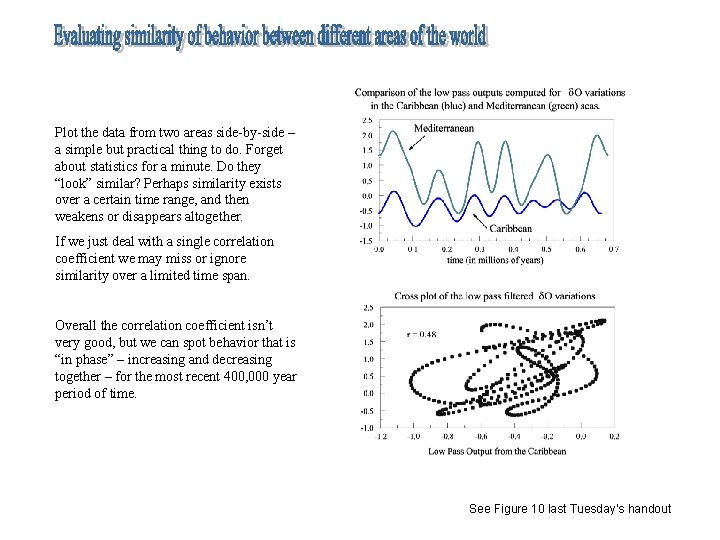
Plot the data from two areas side-by-side – a simple but practical thing to do. Forget about statistics for a minute. Do they “look” similar? Perhaps similarity exists over a certain time range, and then weakens or disappears altogether. If we just deal with a single correlation coefficient we may miss or ignore similarity over a limited time span. Overall the correlation coefficient isn’t very good, but we can spot behavior that is “in phase” – increasing and decreasing together – for the most recent 400, 000 year period of time. See Figure 10 last Tuesday’s handout

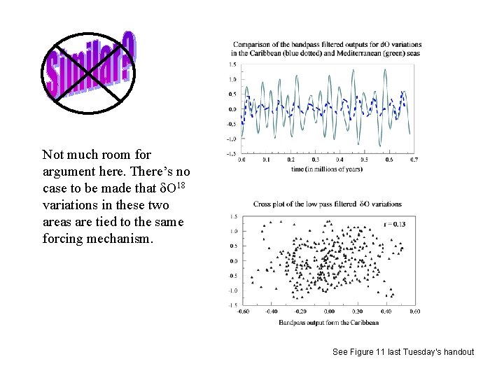
Not much room for argument here. There’s no case to be made that O 18 variations in these two areas are tied to the same forcing mechanism. See Figure 11 last Tuesday’s handout

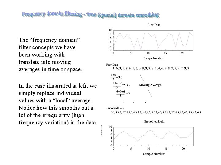
The “frequency domain” filter concepts we have been working with translate into moving averages in time or space. In the case illustrated at left, we simply replace individual values with a “local” average. Notice how this smooths out a lot of the irregularity (high frequency variation) in the data.

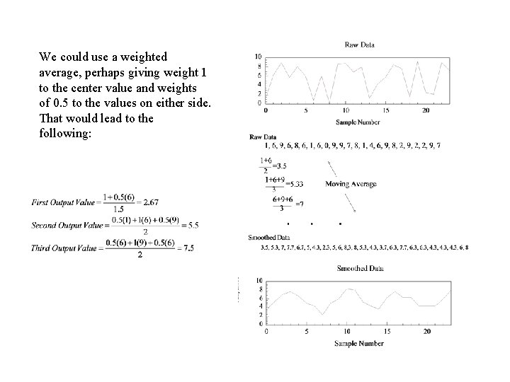
We could use a weighted average, perhaps giving weight 1 to the center value and weights of 0. 5 to the values on either side. That would lead to the following:

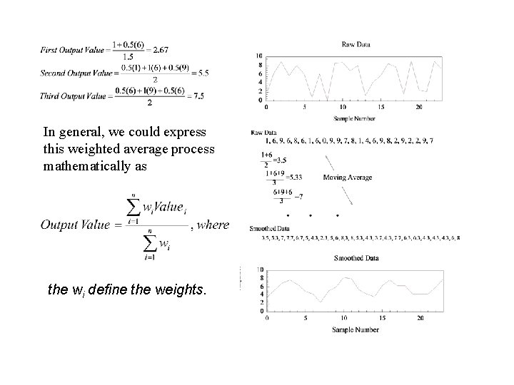
In general, we could express this weighted average process mathematically as the wi define the weights.

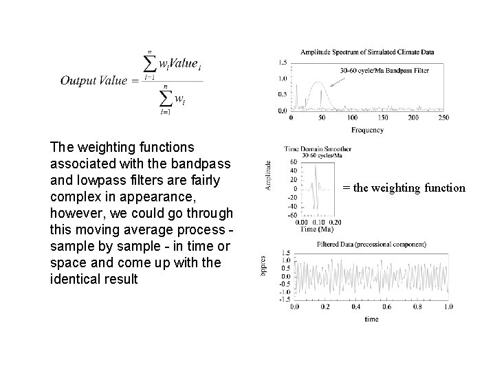
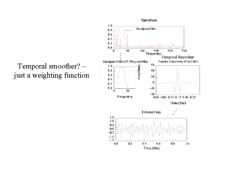
The weighting functions associated with the bandpass and lowpass filters are fairly complex in appearance, however, we could go through this moving average process sample by sample - in time or space and come up with the identical result = the weighting function

Temporal smoother? – just a weighting function

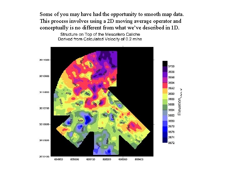
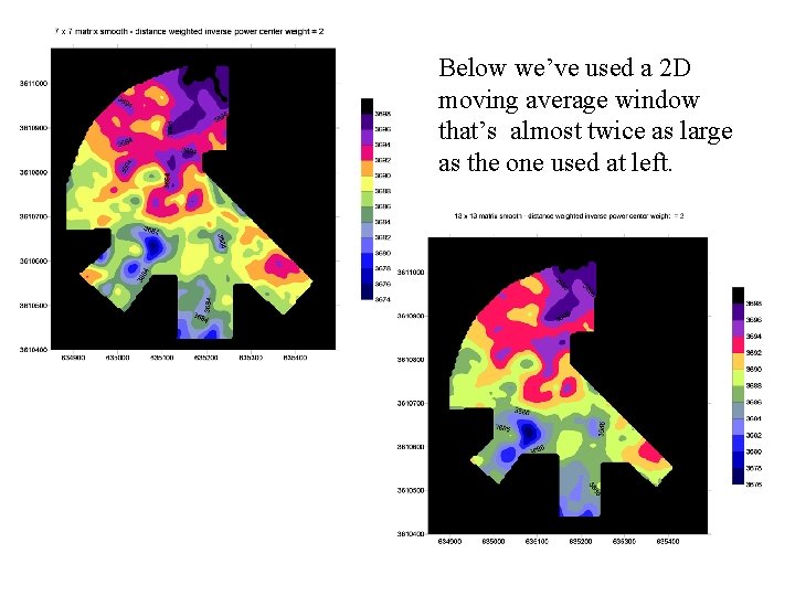
Some of you may have had the opportunity to smooth map data. This process involves using a 2 D moving average operator and conceptually is no different from what we’ve described in 1 D.

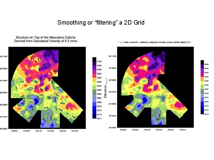
Smoothing or “filtering” a 2 D Grid

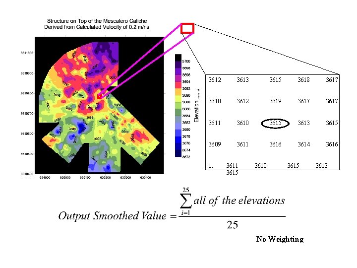
3612 3613 3615 3618 3617 3610 3612 3619 3617 3611 3610 3615 3613 3615 3609 3611 3616 3614 3616 1. 3611 3615 3610 3615 No Weighting 3613

Below we’ve used a 2 D moving average window that’s almost twice as large as the one used at left.

• The spectral analysis problem is due today. • Filter problem set is due on Dec. 4 th • Remember that final project presentations are scheduled for the class exam period – Thursday, Dec. 11 th from 3: 00 to ~ 6: 00 pm. • Bring handouts for all, consisting of a 1 page summary of your project, important references and key figures. • Term reports are due at the time of your presentation.