Todays topics Algorithms Algorithm review Orders of Growth

Today’s topics • Algorithms – Algorithm review – Orders of Growth • Reading: Sections 2. 1 -3. 3 • Upcoming – Integers Comp. Sci 102 © Michael Frank 4. 1

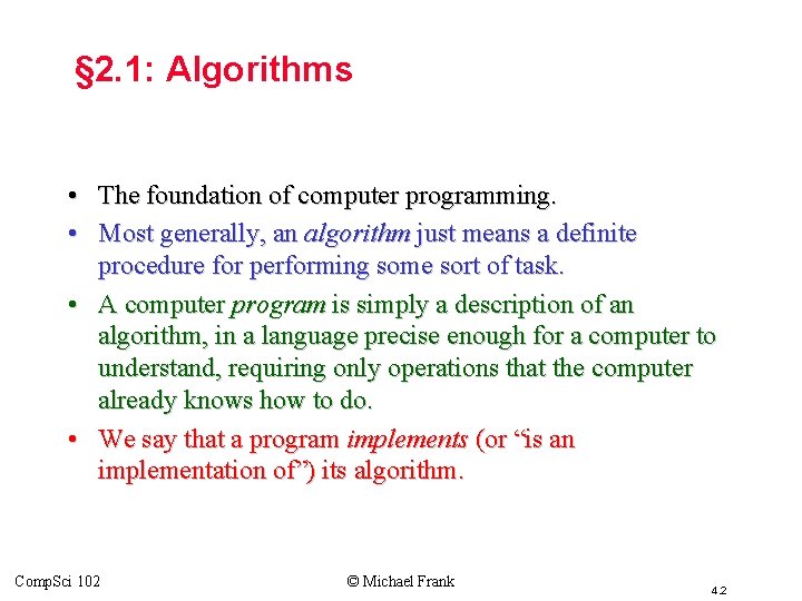
§ 2. 1: Algorithms • The foundation of computer programming. • Most generally, an algorithm just means a definite procedure for performing some sort of task. • A computer program is simply a description of an algorithm, in a language precise enough for a computer to understand, requiring only operations that the computer already knows how to do. • We say that a program implements (or “is an implementation of”) its algorithm. Comp. Sci 102 © Michael Frank 4. 2

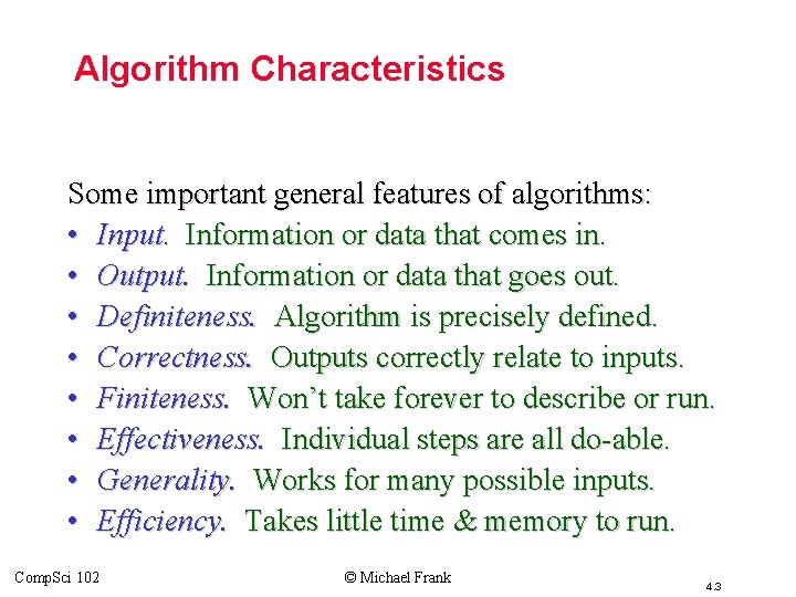
Algorithm Characteristics Some important general features of algorithms: • Input. Information or data that comes in. • Output. Information or data that goes out. • Definiteness. Algorithm is precisely defined. • Correctness. Outputs correctly relate to inputs. • Finiteness. Won’t take forever to describe or run. • Effectiveness. Individual steps are all do-able. • Generality. Works for many possible inputs. • Efficiency. Takes little time & memory to run. Comp. Sci 102 © Michael Frank 4. 3

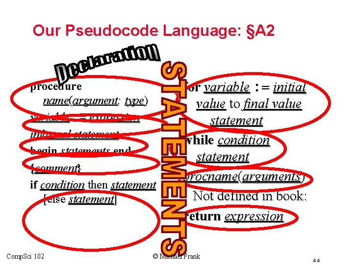
Our Pseudocode Language: §A 2 procedure name(argument: type) variable : = expression informal statement begin statements end {comment} if condition then statement [else statement] Comp. Sci 102 for variable : = initial value to final value statement while condition statement procname(arguments) Not defined in book: return expression © Michael Frank 4. 4

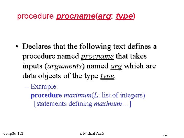
procedure procname(arg: type) • Declares that the following text defines a procedure named procname that takes inputs (arguments) named arg which are data objects of the type. – Example: procedure maximum(L: list of integers) [statements defining maximum…] Comp. Sci 102 © Michael Frank 4. 5

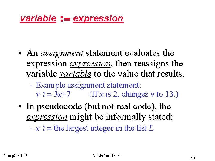
variable : = expression • An assignment statement evaluates the expression, then reassigns the variable to the value that results. – Example assignment statement: v : = 3 x+7 (If x is 2, changes v to 13. ) • In pseudocode (but not real code), the expression might be informally stated: – x : = the largest integer in the list L Comp. Sci 102 © Michael Frank 4. 6

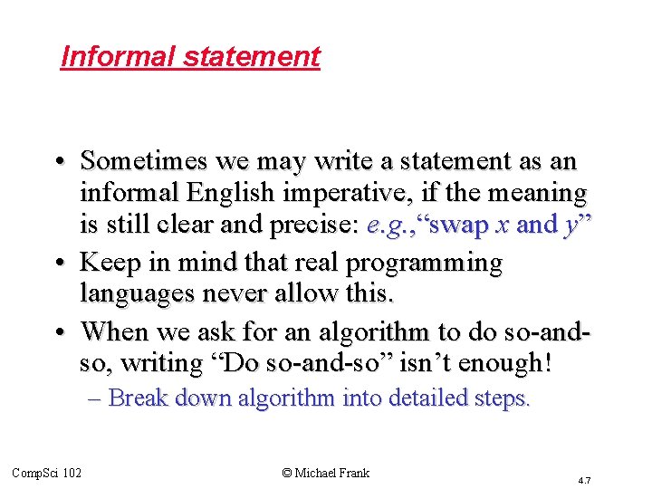
Informal statement • Sometimes we may write a statement as an informal English imperative, if the meaning is still clear and precise: e. g. , “swap x and y” • Keep in mind that real programming languages never allow this. • When we ask for an algorithm to do so-andso, writing “Do so-and-so” isn’t enough! – Break down algorithm into detailed steps. Comp. Sci 102 © Michael Frank 4. 7

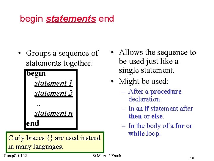
begin statements end • Groups a sequence of statements together: begin statement 1 statement 2 … statement n end • Allows the sequence to be used just like a single statement. • Might be used: Curly braces {} are used instead in many languages. Comp. Sci 102 © Michael Frank – After a procedure declaration. – In an if statement after then or else. – In the body of a for or while loop. 4. 8

{comment} • Not executed (does nothing). • Natural-language text explaining some aspect of the procedure to human readers. • Also called a remark in some real programming languages, e. g. BASIC. • Example, might appear in a max program: – {Note that v is the largest integer seen so far. } Comp. Sci 102 © Michael Frank 4. 9

if condition then statement • Evaluate the propositional expression condition. – If the resulting truth value is True, then execute the statement; – otherwise, just skip on ahead to the next statement after the if statement. • Variant: if cond then stmt 1 else stmt 2 – Like before, but iff truth value is False, executes stmt 2. Comp. Sci 102 © Michael Frank 4. 10

while condition statement • Evaluate the propositional (Boolean) expression condition. • If the resulting value is True, then execute statement. • Continue repeating the above two actions over and over until finally the condition evaluates to False; then proceed to the next statement. Comp. Sci 102 © Michael Frank 4. 11

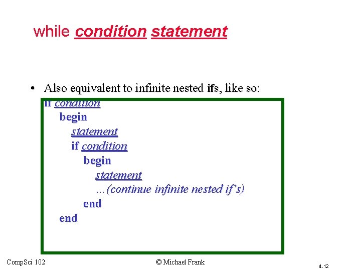
while condition statement • Also equivalent to infinite nested ifs, like so: if condition begin statement …(continue infinite nested if’s) end Comp. Sci 102 © Michael Frank 4. 12

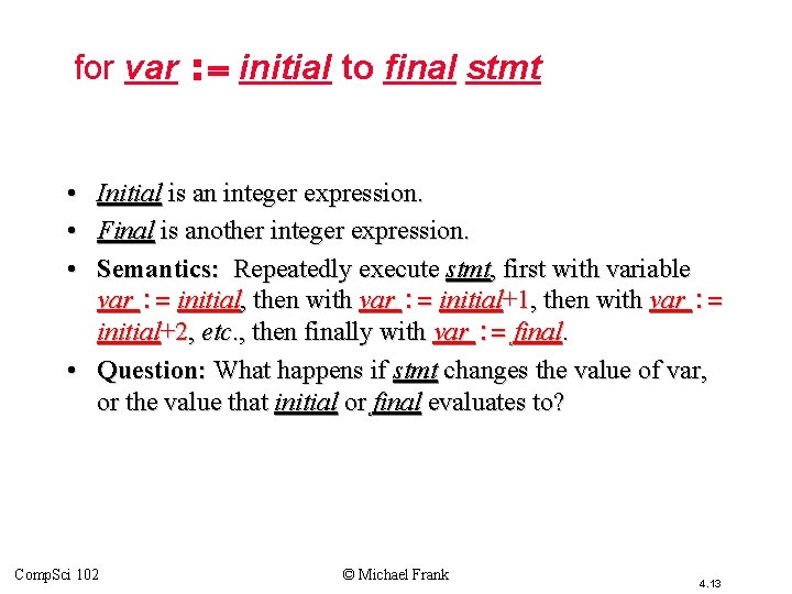
for var : = initial to final stmt • • • Initial is an integer expression. Final is another integer expression. Semantics: Repeatedly execute stmt, first with variable var : = initial, then with var : = initial+1, then with var : = initial+2, etc. , then finally with var : = final. • Question: What happens if stmt changes the value of var, or the value that initial or final evaluates to? Comp. Sci 102 © Michael Frank 4. 13

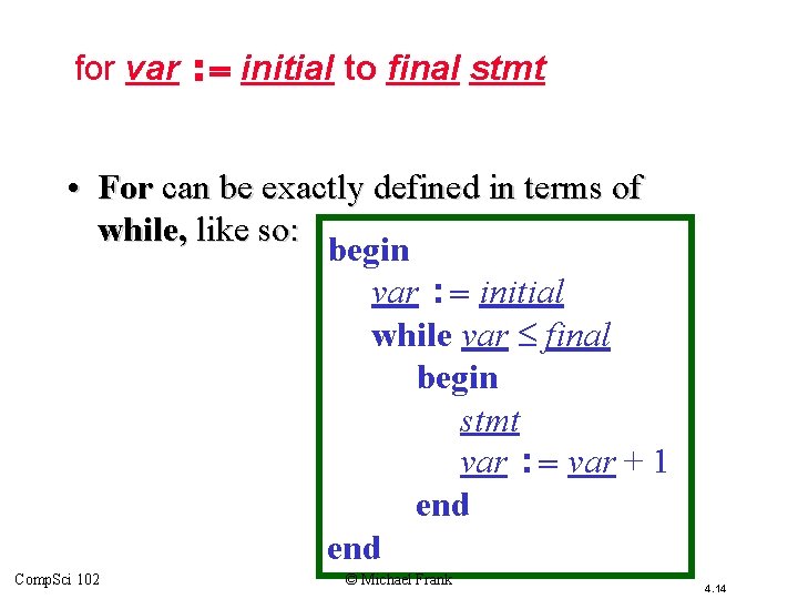
for var : = initial to final stmt • For can be exactly defined in terms of while, like so: begin var : = initial while var final begin stmt var : = var + 1 end Comp. Sci 102 © Michael Frank 4. 14

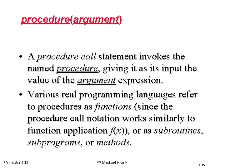
procedure(argument) • A procedure call statement invokes the named procedure, giving it as its input the value of the argument expression. • Various real programming languages refer to procedures as functions (since the procedure call notation works similarly to function application f(x)), or as subroutines, subprograms, or methods. Comp. Sci 102 © Michael Frank 4. 15

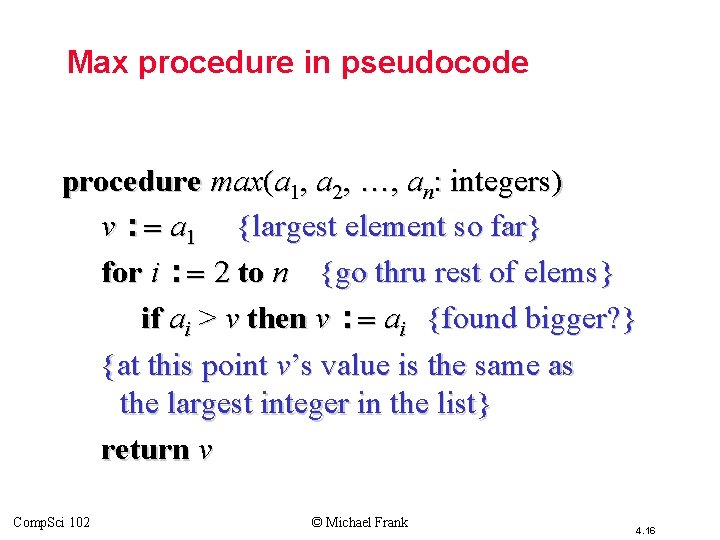
Max procedure in pseudocode procedure max(a 1, a 2, …, an: integers) v : = a 1 {largest element so far} for i : = 2 to n {go thru rest of elems} if ai > v then v : = ai {found bigger? } {at this point v’s value is the same as the largest integer in the list} return v Comp. Sci 102 © Michael Frank 4. 16

Inventing an Algorithm • Requires a lot of creativity and intuition – Like writing proofs. • Unfortunately, we can’t give you an algorithm for inventing algorithms. – Just look at lots of examples… – And practice (preferably, on a computer) – And look at more examples… – And practice some more… etc. , etc. Comp. Sci 102 © Michael Frank 4. 17

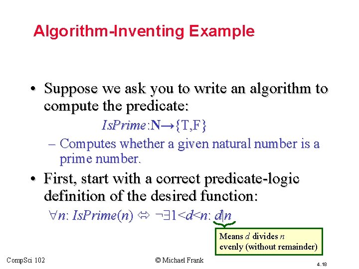
Algorithm-Inventing Example • Suppose we ask you to write an algorithm to compute the predicate: Is. Prime: N→{T, F} – Computes whether a given natural number is a prime number. • First, start with a correct predicate-logic definition of the desired function: n: Is. Prime(n) ¬ 1<d<n: d|n Means d divides n evenly (without remainder) Comp. Sci 102 © Michael Frank 4. 18

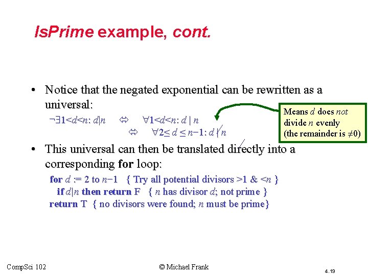
Is. Prime example, cont. • Notice that the negated exponential can be rewritten as a universal: Means d does not ¬ 1<d<n: d|n 1<d<n: d | n 2≤ d ≤ n− 1: d | n divide n evenly (the remainder is ≠ 0) • This universal can then be translated directly into a corresponding for loop: for d : = 2 to n− 1 { Try all potential divisors >1 & <n } if d|n then return F { n has divisor d; not prime } return T { no divisors were found; n must be prime} Comp. Sci 102 © Michael Frank 4. 19

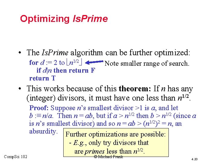
Optimizing Is. Prime • The Is. Prime algorithm can be further optimized: for d : = 2 to n 1/2 if d|n then return F return T Note smaller range of search. • This works because of this theorem: If n has any (integer) divisors, it must have one less than n 1/2. Comp. Sci 102 Proof: Suppose n’s smallest divisor >1 is a, and let b : ≡ n/a. Then n = ab, but if a > n 1/2 then b > n 1/2 (since a is n’s smallest divisor) and so n = ab > (n 1/2)2 = n, an absurdity. Further optimizations are possible: - E. g. , only try divisors that are primes less than n 1/2. © Michael Frank 4. 20

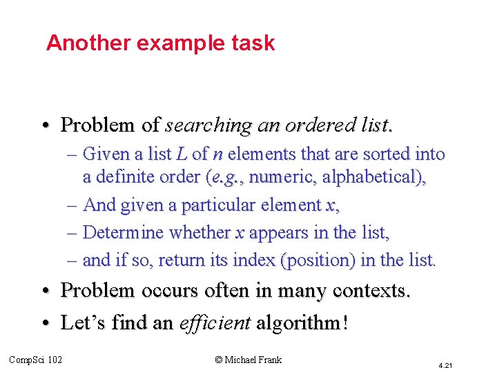
Another example task • Problem of searching an ordered list. – Given a list L of n elements that are sorted into a definite order (e. g. , numeric, alphabetical), – And given a particular element x, – Determine whether x appears in the list, – and if so, return its index (position) in the list. • Problem occurs often in many contexts. • Let’s find an efficient algorithm! Comp. Sci 102 © Michael Frank 4. 21

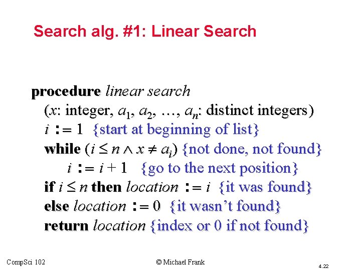
Search alg. #1: Linear Search procedure linear search (x: integer, a 1, a 2, …, an: distinct integers) i : = 1 {start at beginning of list} while (i n x ai) {not done, not found} i : = i + 1 {go to the next position} if i n then location : = i {it was found} else location : = 0 {it wasn’t found} return location {index or 0 if not found} Comp. Sci 102 © Michael Frank 4. 22

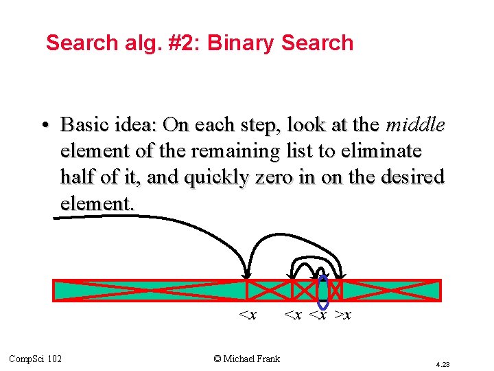
Search alg. #2: Binary Search • Basic idea: On each step, look at the middle element of the remaining list to eliminate half of it, and quickly zero in on the desired element. <x Comp. Sci 102 © Michael Frank <x <x >x 4. 23

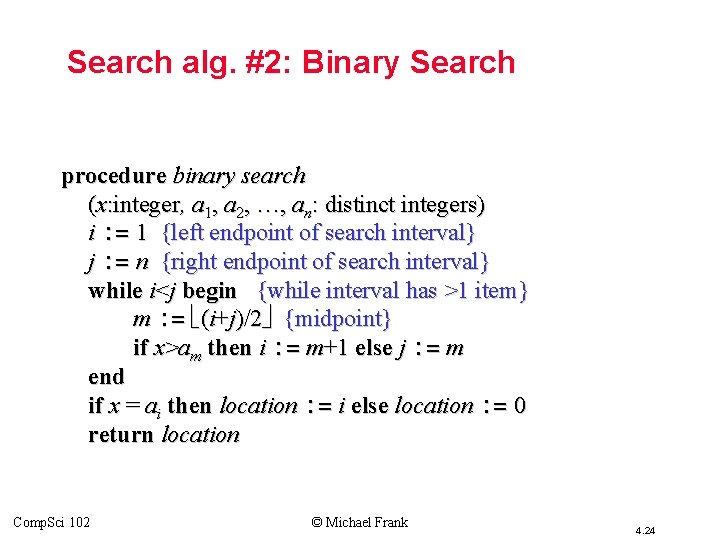
Search alg. #2: Binary Search procedure binary search (x: integer, a 1, a 2, …, an: distinct integers) i : = 1 {left endpoint of search interval} j : = n {right endpoint of search interval} while i<j begin {while interval has >1 item} m : = (i+j)/2 {midpoint} if x>am then i : = m+1 else j : = m end if x = ai then location : = i else location : = 0 return location Comp. Sci 102 © Michael Frank 4. 24

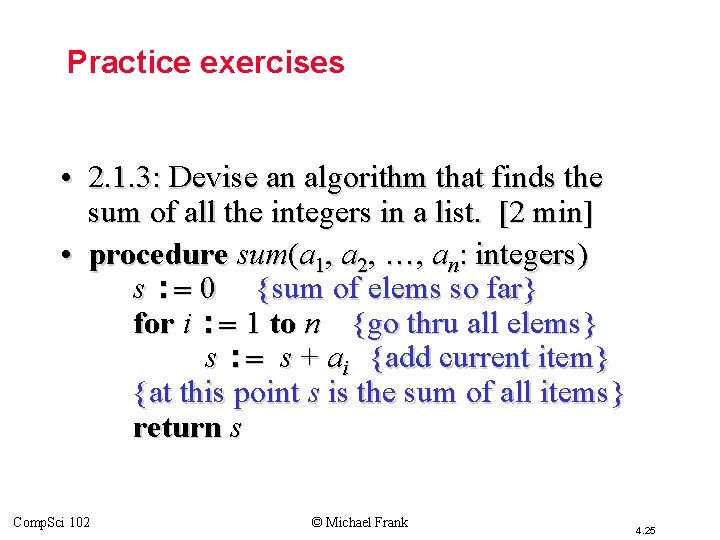
Practice exercises • 2. 1. 3: Devise an algorithm that finds the sum of all the integers in a list. [2 min] • procedure sum(a 1, a 2, …, an: integers) s : = 0 {sum of elems so far} for i : = 1 to n {go thru all elems} s : = s + ai {add current item} {at this point s is the sum of all items} return s Comp. Sci 102 © Michael Frank 4. 25

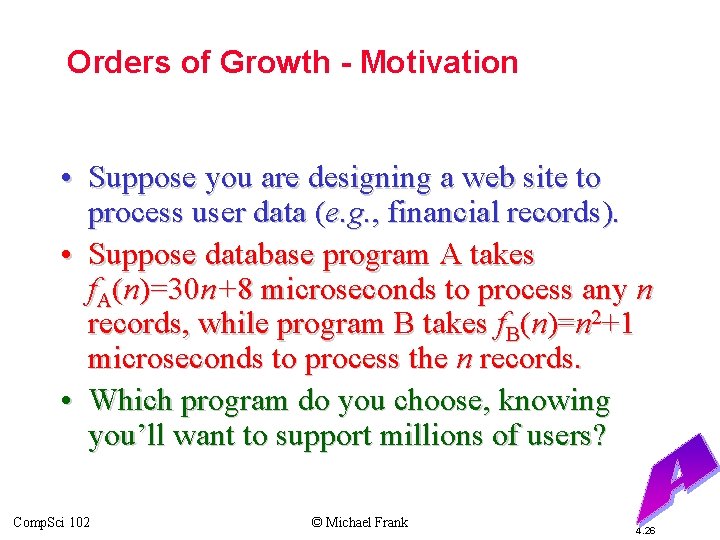
Orders of Growth - Motivation • Suppose you are designing a web site to process user data (e. g. , financial records). • Suppose database program A takes f. A(n)=30 n+8 microseconds to process any n records, while program B takes f. B(n)=n 2+1 microseconds to process the n records. • Which program do you choose, knowing you’ll want to support millions of users? Comp. Sci 102 © Michael Frank 4. 26

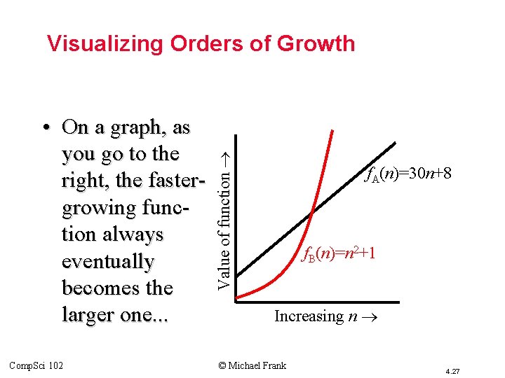
• On a graph, as you go to the right, the fastergrowing function always eventually becomes the larger one. . . Comp. Sci 102 Value of function Visualizing Orders of Growth f. A(n)=30 n+8 f. B(n)=n 2+1 Increasing n © Michael Frank 4. 27

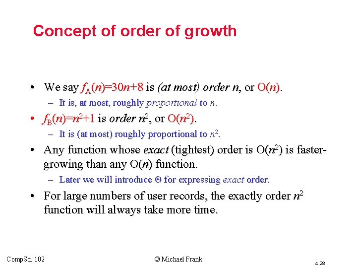
Concept of order of growth • We say f. A(n)=30 n+8 is (at most) order n, or O(n). – It is, at most, roughly proportional to n. • f. B(n)=n 2+1 is order n 2, or O(n 2). – It is (at most) roughly proportional to n 2. • Any function whose exact (tightest) order is O(n 2) is fastergrowing than any O(n) function. – Later we will introduce Θ for expressing exact order. • For large numbers of user records, the exactly order n 2 function will always take more time. Comp. Sci 102 © Michael Frank 4. 28

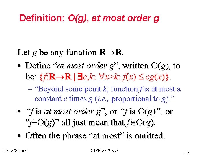
Definition: O(g), at most order g Let g be any function R R. • Define “at most order g”, written O(g), to be: {f: R R | c, k: x>k: f(x) cg(x)}. – “Beyond some point k, function f is at most a constant c times g (i. e. , proportional to g). ” • “f is at most order g”, or “f is O(g)”, or “f=O(g)” all just mean that f O(g). • Often the phrase “at most” is omitted. Comp. Sci 102 © Michael Frank 4. 29

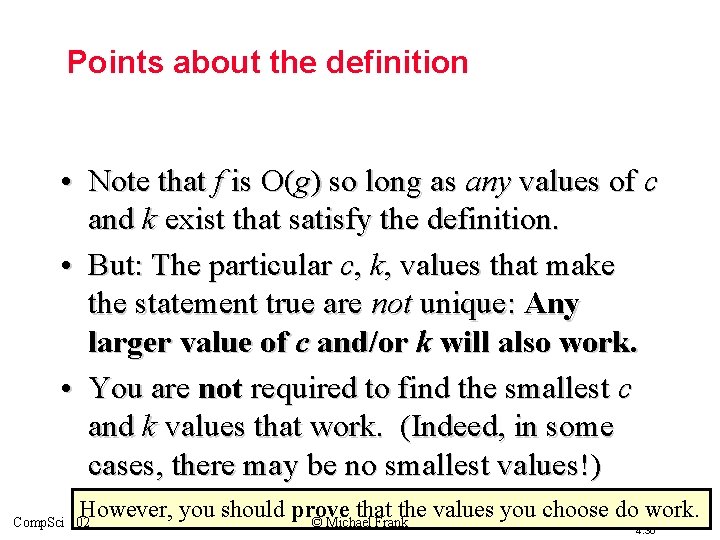
Points about the definition • Note that f is O(g) so long as any values of c and k exist that satisfy the definition. • But: The particular c, k, values that make the statement true are not unique: Any larger value of c and/or k will also work. • You are not required to find the smallest c and k values that work. (Indeed, in some cases, there may be no smallest values!) However, you should prove that the values you choose do work. © Michael Frank Comp. Sci 102 4. 30

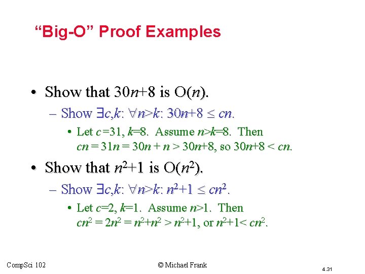
“Big-O” Proof Examples • Show that 30 n+8 is O(n). – Show c, k: n>k: 30 n+8 cn. • Let c=31, k=8. Assume n>k=8. Then cn = 31 n = 30 n + n > 30 n+8, so 30 n+8 < cn. • Show that n 2+1 is O(n 2). – Show c, k: n>k: n 2+1 cn 2. • Let c=2, k=1. Assume n>1. Then cn 2 = 2 n 2 = n 2+n 2 > n 2+1, or n 2+1< cn 2. Comp. Sci 102 © Michael Frank 4. 31

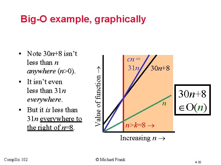
Big-O example, graphically cn = 31 n Value of function • Note 30 n+8 isn’t less than n anywhere (n>0). • It isn’t even less than 31 n everywhere. • But it is less than 31 n everywhere to the right of n=8. 30 n+8 n 30 n+8 O(n) n>k=8 Increasing n Comp. Sci 102 © Michael Frank 4. 32

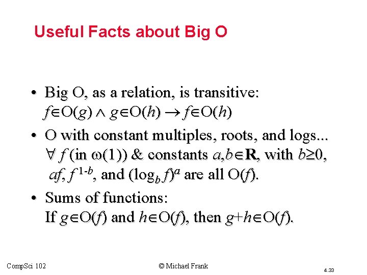
Useful Facts about Big O • Big O, as a relation, is transitive: f O(g) g O(h) f O(h) • O with constant multiples, roots, and logs. . . f (in (1)) & constants a, b R, with b 0, af, f 1 -b, and (logb f)a are all O(f). • Sums of functions: If g O(f) and h O(f), then g+h O(f). Comp. Sci 102 © Michael Frank 4. 33

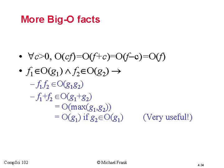
More Big-O facts • c>0, O(cf)=O(f+c)=O(f) • f 1 O(g 1) f 2 O(g 2) – f 1 f 2 O(g 1 g 2) – f 1+f 2 O(g 1+g 2) = O(max(g 1, g 2)) = O(g 1) if g 2 O(g 1) Comp. Sci 102 © Michael Frank (Very useful!) 4. 34

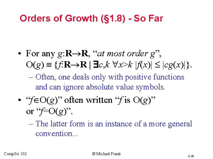
Orders of Growth (§ 1. 8) - So Far • For any g: R R, “at most order g”, O(g) {f: R R | c, k x>k |f(x)| |cg(x)|}. – Often, one deals only with positive functions and can ignore absolute value symbols. • “f O(g)” often written “f is O(g)” or “f=O(g)”. – The latter form is an instance of a more general convention. . . Comp. Sci 102 © Michael Frank 4. 35

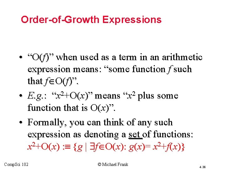
Order-of-Growth Expressions • “O(f)” when used as a term in an arithmetic expression means: “some function f such that f O(f)”. • E. g. : “x 2+O(x)” means “x 2 plus some function that is O(x)”. • Formally, you can think of any such expression as denoting a set of functions: x 2+O(x) : {g | f O(x): g(x)= x 2+f(x)} Comp. Sci 102 © Michael Frank 4. 36

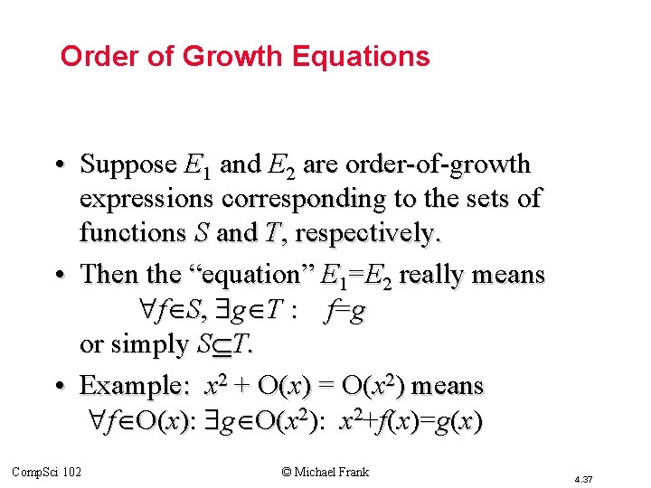
Order of Growth Equations • Suppose E 1 and E 2 are order-of-growth expressions corresponding to the sets of functions S and T, respectively. • Then the “equation” E 1=E 2 really means f S, g T : f=g or simply S T. • Example: x 2 + O(x) = O(x 2) means f O(x): g O(x 2): x 2+f(x)=g(x) Comp. Sci 102 © Michael Frank 4. 37

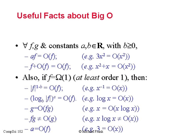
Useful Facts about Big O • f, g & constants a, b R, with b 0, – af = O(f); – f+O(f) = O(f); (e. g. 3 x 2 = O(x 2)) (e. g. x 2+x = O(x 2)) • Also, if f= (1) (at least order 1), then: – |f|1 -b = O(f); (e. g. x 1 = O(x)) – (logb |f|)a = O(f). (e. g. log x = O(x)) – g=O(fg) (e. g. x = O(x log x)) – fg O(g) (e. g. x log x O(x)) – a=O(f) (e. g. 3 = O(x)) Comp. Sci 102 © Michael Frank 4. 38

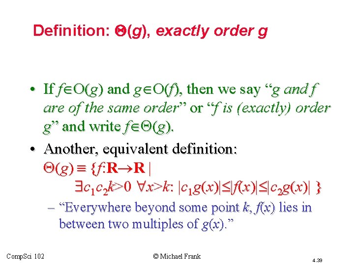
Definition: (g), exactly order g • If f O(g) and g O(f), then we say “g and f are of the same order” or “f is (exactly) order g” and write f (g). • Another, equivalent definition: (g) {f: R R | c 1 c 2 k>0 x>k: |c 1 g(x)| |f(x)| |c 2 g(x)| } – “Everywhere beyond some point k, f(x) lies in between two multiples of g(x). ” Comp. Sci 102 © Michael Frank 4. 39

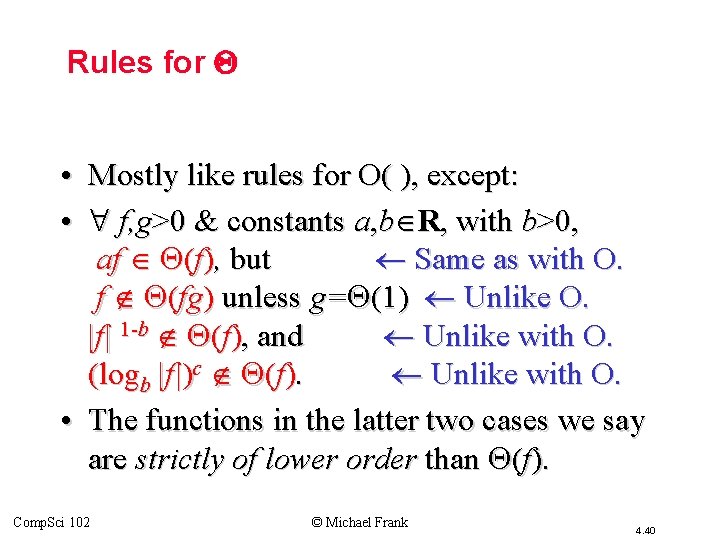
Rules for • Mostly like rules for O( ), except: • f, g>0 & constants a, b R, with b>0, af (f), but Same as with O. f (fg) unless g= (1) Unlike O. |f| 1 -b (f), and Unlike with O. (logb |f|)c (f). Unlike with O. • The functions in the latter two cases we say are strictly of lower order than (f). Comp. Sci 102 © Michael Frank 4. 40

example • Determine whether: • Quick solution: Comp. Sci 102 © Michael Frank 4. 41

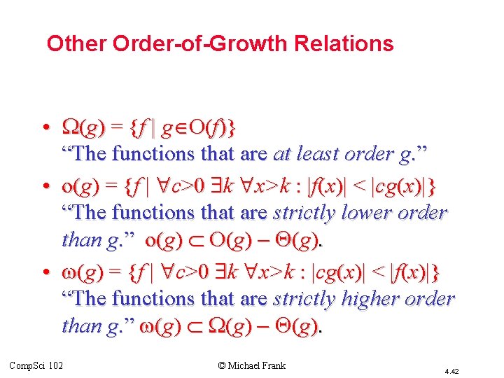
Other Order-of-Growth Relations • (g) = {f | g O(f)} “The functions that are at least order g. ” • o(g) = {f | c>0 k x>k : |f(x)| < |cg(x)|} “The functions that are strictly lower order than g. ” o(g) O(g) (g). • (g) = {f | c>0 k x>k : |cg(x)| < |f(x)|} “The functions that are strictly higher order than g. ” (g). Comp. Sci 102 © Michael Frank 4. 42

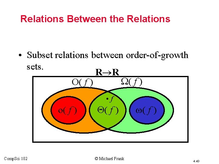
Relations Between the Relations • Subset relations between order-of-growth sets. R R ( f ) O( f ) • f o( f ) Comp. Sci 102 ( f ) © Michael Frank ( f ) 4. 43

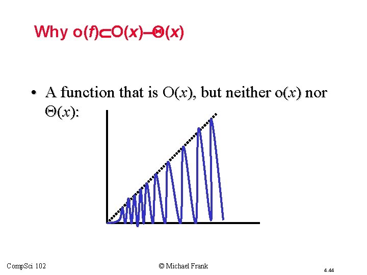
Why o(f) O(x) • A function that is O(x), but neither o(x) nor (x): Comp. Sci 102 © Michael Frank 4. 44

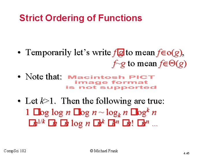
Strict Ordering of Functions • Temporarily let’s write f� g to mean f o(g), f~g to mean f (g) • Note that: • Let k>1. Then the following are true: 1 �log n ~ logk n �n 1/k �n �n log n �nk �kn �n! �nn … Comp. Sci 102 © Michael Frank 4. 45

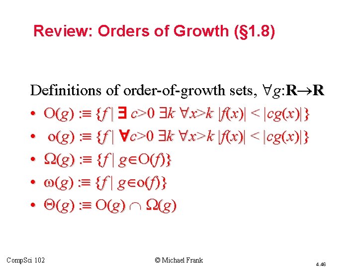
Review: Orders of Growth (§ 1. 8) Definitions of order-of-growth sets, g: R R • O(g) : {f | c>0 k x>k |f(x)| < |cg(x)|} • o(g) : {f | c>0 k x>k |f(x)| < |cg(x)|} • (g) : {f | g O(f)} • (g) : {f | g o(f)} • (g) : O(g) Comp. Sci 102 © Michael Frank 4. 46