Todays lesson Chapter 12 Paired experimental designs Paired

Today’s lesson (Chapter 12) • Paired experimental designs • Paired t-test • Confidence interval for E(W-Y)

Paired Design • Find two experimental units that are more like each other than randomly selected units. – Two animals from the same litter – Before and after measurements on the same subject. • Apply the A treatment to one unit randomly selected and the B treatment to the other.

Analysis of Paired Design • There are n pairs of experimental units. • For unit i, Wi represents the A treatment observation from the i-th pair. • For unit i, Yi represents the B treatment observation from the i-th pair. • Calculate the difference Di=Wi-Yi. • Do a one-sample t-test on the differences.

Analysis of Paired Design • That is, null hypothesis is E(W-Y)=0. • Alternative hypothesis may be left, right, or two-sided. • Test statistic is the mean of the differences. • Estimated standard error of the mean difference is the standard deviation of the D values divided by the square root of n. • Standardize the test statistic as usual.

Example Problem 1 • A research team evaluated a medicine to determine whether it lowered a blood component. They measured B, the amount of the component in six patients before a protocol using the medicine was followed and then measured A, the amount of the component after the administration of the medicine.

Example Problem 1 • They wished to test the null hypothesis that E(A)=E(B) against the alternative that E(A)<E(B). Their experimental results are given in the following table. Which of the following is a correct decision? • Usual options: reject at 0. 01 level, accept at 0. 01 and reject at 0. 05, accept at 0. 05 and reject at 0. 10, accept at 0. 10.

Data for Problem 1

Solution of Problem 1 • Recognize that this problem requires a paired t-test (before and after comparison). • Compute the six differences A-B: – -20, -30, -40, -30, -10, -50. • Compute mean difference – sum of differences is -180 – mean difference is -30

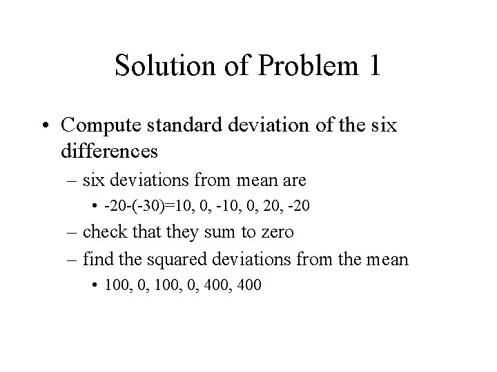
Solution of Problem 1 • Compute standard deviation of the six differences – six deviations from mean are • -20 -(-30)=10, 0, -10, 0, 20, -20 – check that they sum to zero – find the squared deviations from the mean • 100, 0, 400, 400

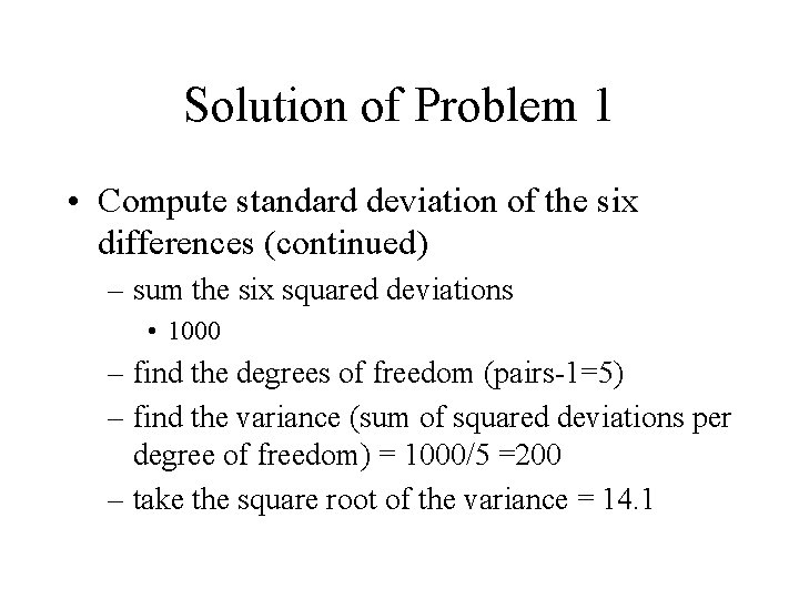
Solution of Problem 1 • Compute standard deviation of the six differences (continued) – sum the six squared deviations • 1000 – find the degrees of freedom (pairs-1=5) – find the variance (sum of squared deviations per degree of freedom) = 1000/5 =200 – take the square root of the variance = 14. 1

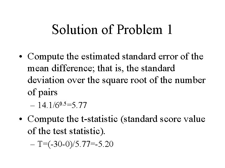
Solution of Problem 1 • Compute the estimated standard error of the mean difference; that is, the standard deviation over the square root of the number of pairs – 14. 1/60. 5=5. 77 • Compute the t-statistic (standard score value of the test statistic). – T=(-30 -0)/5. 77=-5. 20

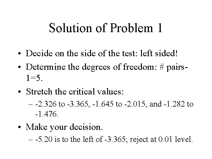
Solution of Problem 1 • Decide on the side of the test: left sided! • Determine the degrees of freedom: # pairs 1=5. • Stretch the critical values: – -2. 326 to -3. 365, -1. 645 to -2. 015, and -1. 282 to -1. 476. • Make your decision. – -5. 20 is to the left of -3. 365; reject at 0. 01 level.

Most Fundamental Design Advice • Pair what you can, randomize what you cannot. • That is, always used a paired design when possible. • There is a generalization of a pair. It is called a block. • ADVICE: Block what you can, randomize what you cannot.

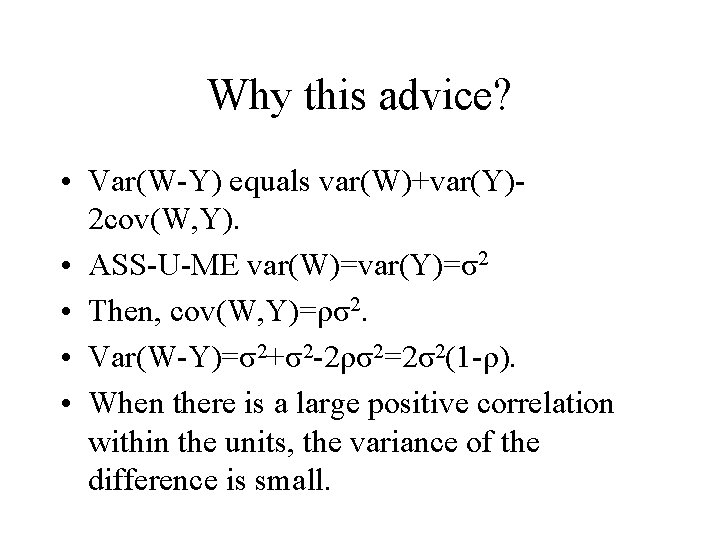
Why this advice? • Var(W-Y) equals var(W)+var(Y)2 cov(W, Y). • ASS-U-ME var(W)=var(Y)=σ2 • Then, cov(W, Y)=ρσ2. • Var(W-Y)=σ2+σ2 -2ρσ2=2σ2(1 -ρ). • When there is a large positive correlation within the units, the variance of the difference is small.

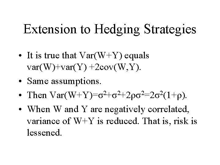
Extension to Hedging Strategies • It is true that Var(W+Y) equals var(W)+var(Y) +2 cov(W, Y). • Same assumptions. • Then Var(W+Y)=σ2+σ2+2ρσ2=2σ2(1+ρ). • When W and Y are negatively correlated, variance of W+Y is reduced. That is, risk is lessened.

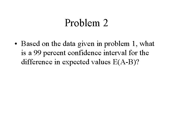
Problem 2 • Based on the data given in problem 1, what is a 99 percent confidence interval for the difference in expected values E(A-B)?

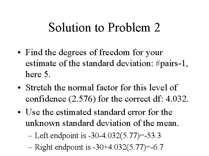
Solution to Problem 2 • Find the degrees of freedom for your estimate of the standard deviation: #pairs-1, here 5. • Stretch the normal factor for this level of confidence (2. 576) for the correct df: 4. 032. • Use the estimated standard error for the unknown standard deviation of the mean. – Left endpoint is -30 -4. 032(5. 77)=-53. 3 – Right endpoint is -30+4. 032(5. 77)=-6. 7

Using SPSS to get paired t-test • Statistics, compare means, paired t-test.

Example Computer Problem • Two statistical procedures exist to determine the estimated location of a gene. • Which procedure comes closer to the correct location of the gene? • Use the results of a simulation study to answer the question.

Data of Study • Genetic model specified (recessive, all families affected by the same genetic pattern --no heterogeneity). • Use simulation to generate the results of 100 independent studies. • Apply two statistics (maximum hlod and Kong and Cox correct to the Nonparametric Linkage (NPL) statistic of Genehunter) to each study.

Design of the Comparison • For each of the 100 replicates, calculate the difference D of the distance from the maximum hlod analysis and the distance from the maximum NPL statistic. • Use paired t-test to test the null hypothesis that the expected distance using the maximum hlod is the same as the expected distance using the maximum NPL. • Closer is better.

Results • Maximum hlod is significantly closer than the maximum NPL for this genetic model.

Summary • Paired t-test design • Discussion of why paired t-test likely to be better. • Block what you can, randomize what you cannot. • Illustrated computations of the paired t-test on both test and confidence interval.