tm Sensible Heat Flux Slide presentation Part Three

tm “Sensible Heat Flux ” Slide presentation Part Three

Surface Energy Budget Equation Rn = G + H + ET ET = Rn – G – H Note that ordinarily, we cover the calculation of Rn and G prior to H. However, for the training models, we will cover H first, since that model (F 06) computes an adjusted albedo (for ‘tall vegetation’) that is required for input to the Rn and G model (F 07). Therefore Rn and G are covered later. Rn H ET G

Sensible Heat Flux is an Aerodynamic Process

Hollister Sage Brush site – Installed Feb. 2010 3 1 16 32 20 7 2 2 3 -D sonic anenometers Li. Cor 7500 H 20/CO 2 Infrared Net radiometers Scintec BLS 900 Scintillometer Soil Heat Flux Sensors Soil Temperature Sensors Soil Water Content Sensors Soil Water Potential Sensors Rain Gages Infrared Temperature Sensors

Sensible Heat Flux is an Aerodynamic Process Tens of Soil Heat Flux Sensors for Spatial Sampling and Reduancy with the eddy covariance system

FLUX OF HEAT AND VAPOR INTO THE AIR OVER SAGEBRUSH Scintillometer vs. Eddy Covariance

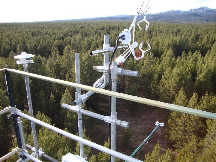
Raft River Cheatgrass site – Installed Nov. 2009 2 1 3 1 16 32 20 7 2 2 3 -D sonic anenometers Li. Cor 7500 H 20/CO 2 Infrared A. Net radiometers Scintec BLS 900 Scintillometer Soil Heat Flux Sensors Soil Temperature Sensors Soil Water Content Sensors Soil Water Potential Sensors Rain Gages Infrared Temperature Sensors

Island Park Lodgepole Pine site – Installed Oct. 2010 2 2 7 1 24 48 32 2 3 -D sonic anenometers Li. Cor 7500 H 20/CO 2 Infrared A. Net radiometers Scintec BLS 900 Scintillometer Soil Heat Flux Sensors Soil Temperature Sensors Soil Water Content Sensors Rain Gages Sonic Snow Depth Sensors Infrared Temperature Sensors

Evapotranspiration – 2006 -- from METRIC Surface Energy Balance Island Park Trans

South Tower w/ Scintillometer Receiver North Tower w/ Scintillometer Transmitter

Sensible Heat Flux (H) – “Traditional Approach” H = cp (Taero - Tair) / rah Challenge (BIAS): Up to 2 K different from Trad (satellite) Taero = aerodynamic temperature rah = the aerodynamic resistance Challenge (BIAS): Unknown Spatial Distrib. of Tair (feedback between H, Trad, Tair) z 2 Tair rah H u* = friction velocity k = von karmon constant (0. 41) ψh = buoyancy-instability correction = f(H) z 1 Taero

Sensible Heat Flux (H) – SEBAL and METRIC H = ( × cp × d. T) / Advantage: d. T is inverse calibrated (simulated) (free of Trad vs. Taero and free of Tair) Advantage: d. T and rah ‘float’ above the surface and are ‘free’ of rah zoh and some limitations of a single source approach d. T = “floating” near surface temperature difference (K) rah = the aerodynamic resistance from z 1 to z 2 d. T z 1 u* = friction velocity k = von karmon constant (0. 41) rah H

Friction Velocity (u*) for neutral profiles: ux is wind speed (m/s) at height zx above ground. zom is the momentum roughness length (m). zom can be calculated in different ways: – For agricultural areas: zom = 0. 12 height of vegetation (h) – From a land-use map – As a function of NDVI and surface albedo for unstable profiles:

Zero Plane Displacement (d) and Momentum Roughness Length (zom) The wind speed goes to zero at the height (d + zom).

Calculation of Aerodynamic Resistance (rah) z 2 = 2. 0 m, T 2 = T 2 m z 1 = 0. 1 m, T 1 = T 0. 01 m (z 1 = 0. 1 m in METRIC, 0. 01 m in SEBA

Atmospheric Stability

Stability Correction for u*and rah • • New values for d. T are computed for the “anchor” pixels. New values for a and b are computed. A corrected value for H is computed. The stability correction is repeated until H stabilizes.

Iterative Process to Compute H Weather station u, zx, zom , u* H for each pixel wind speed at 200 meters m (blending) friction velocity at each pixel h (z 1) rah for each pixel Cold Pixel Hot Pixel Hcold=Rn-G- ETcold Hhot=Rn-G-λEThot d. Tcold=Hcold*rah/( Cp) d. Thot = Hhot*rah /( Cp) d. T for each pixel d. T=a. Ts+b h (z 2)

Aerodynamic Equations used in METRICtm H = ( ρ cp)(Ta 1 – Ta 1 ) / rah Ta 1 – Ta 2 = f (Ts) Correction for atmospheric instability and for stable

tm “Estimating Evaporation for Water using aerodynamics”

Uncertainties in Energy Balance in Open Water (due to G) G (Heat Storage) in Deep, cool lakes can be as large as 0. 5 Rn, variable with time of year, and very uncertain. Therefore, LE from energy balance is quite uncertain for lakes Therefore, an aerodynamic method has been derived in METRIC for water

Evaporation by Energy Balance LE = Rn - Qt - H + Qadvect – Problem: Water is not Opaque like Land Vegetation and Solar Energy penetrates the Surface – Therefore, some of Rn becomes G (called Qt for water) – Qt can be more than one-half as large as Rn – Qt varies with turbidity, water depth, advection into and from water body

Penetration of Solar Radiation Infrared is absorbed near the surface and is not as big a problem as UV, blue, green and red This energy is converted to heat and can stay in the water body, below the surface, for months Evaporation is a surface phenomenon!!!

Aerodynamic equation for Evaporation from open water – new in 2010 E units of mm h-1 ρa is density of air (kg m-3) ρw is density of water (kg m-3) qsat is specific humidity of the air at saturation (kg kg-1) rav is aerodynamic resistance to vapor transfer, s m-1 3600 converts from seconds to hours and the 1000 converts from m to mm Fortunately, water does not have surface (stomatal) resistance like vegetation qa qo E rav

Specific humidity (q) Air density and over ice (used when Ts < ~275 K): Estimation of actual vapor pressure: – assume constant RH over domain qa (same time from sunrise to overpass time) (early morning vapor content is in synch with nighttime temperature everywhere) qo E rav

Aerodynamic resistance Zero plane displacement d can be assumed 0 for water For water, zoh is typically set equal to zom. zbl = blending height (~ 200 m) The stability functions, ψ, for momentum and heat flux are already computed in METRIC

Aerodynamic Roughness for Water Using parameters suggested by Lofgren (2004), the Charnock (1955) relationship yields: for zom in m and u in m/s, where u 10 is wind speed at 10 m height. For METRIC application:

Translation of Instantaneous Evaporation to the day: Use the “Ea” expression of Penman(1948) derived from weather station data, only, where Ea is “pseudo evaporation”: – Ta is air temperature at weather station – qo is saturated specific humidity at air temperature o, q q a – qa is specific humidity of air: Assume that behavior of Ea 24 to Ea inst is same as behavior of E 24 to Einst Ea rav

Development and Testing from American Falls Res. “Official” Univ. Idaho Faculty speed boat 25 miles Evap. Equipment 2004 2. 5 miles 4000 m

3 -D Sonic Anemometer for EC (H) American Falls Reservoir - 2004

REBS Bowen Ratio Sys. (B = H/LE) Therefore and No need to touch the water

Verifying heat flux for reservoirs (Dr. Wim Bastiaanssen, creator of SEBAL)