Timing Model Reduction for Hierarchical Timing Analysis Shuo
![Previous Works • Transform timing graph [Visweswariah ICCAD’ 99, Moon DAC’ 02]. – Perform Previous Works • Transform timing graph [Visweswariah ICCAD’ 99, Moon DAC’ 02]. – Perform](https://slidetodoc.com/presentation_image_h2/34d24ec872dd34e2888617bd624b28a1/image-6.jpg)

- Slides: 30

Timing Model Reduction for Hierarchical Timing Analysis Shuo Zhou Synopsys November 7, 2006

Outline • Static Timing Analysis in Design Flow • Hierarchical timing analysis • Proposed Techniques – Iterative timing model reduction algorithm based on a biclique-star replacement technique. • Experimental Results • Conclusions 2

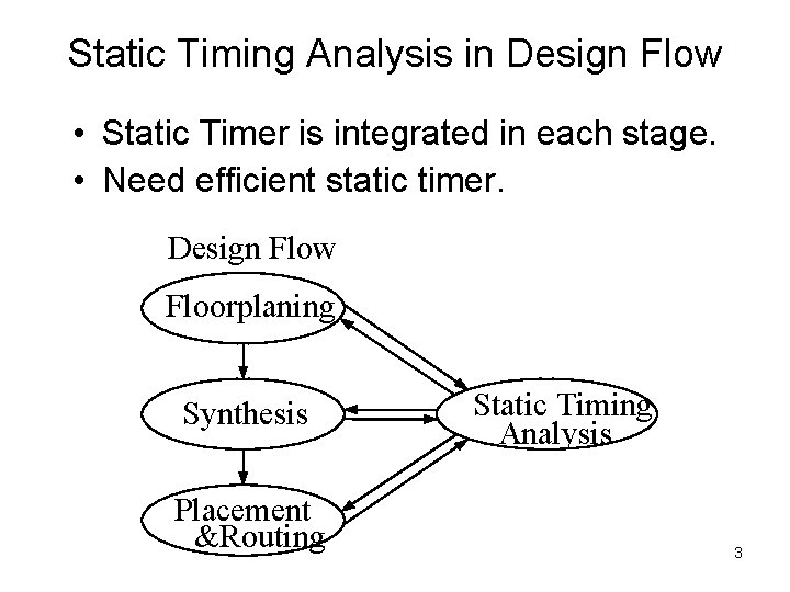
Static Timing Analysis in Design Flow • Static Timer is integrated in each stage. • Need efficient static timer. Design Flow Floorplaning Synthesis Placement &Routing Static Timing Analysis 3

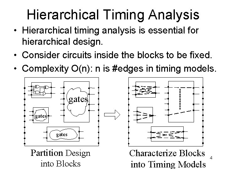
Hierarchical Timing Analysis • Hierarchical timing analysis is essential for hierarchical design. • Consider circuits inside the blocks to be fixed. • Complexity O(n): n is #edges in timing models. gates Partition Design into Blocks Characterize Blocks into Timing Models 4

Problem Statement • Timing model minimization for hierarchical timing analysis: – Given a hierarchical block, construct an abstract timing model with minimal number of edges that covers the longest and shortest path delays of each pair of input and output in the block. 5
![Previous Works Transform timing graph Visweswariah ICCAD 99 Moon DAC 02 Perform Previous Works • Transform timing graph [Visweswariah ICCAD’ 99, Moon DAC’ 02]. – Perform](https://slidetodoc.com/presentation_image_h2/34d24ec872dd34e2888617bd624b28a1/image-6.jpg)
Previous Works • Transform timing graph [Visweswariah ICCAD’ 99, Moon DAC’ 02]. – Perform serial/parallel edge merging. • Represent delay matrix with minimal number of edges. – Optimal realization of a distance matrix [Hakimi Quart. Appl. Math. 22 (1964), Chung http: //www. math. ucsd. edu/˜fan]. – Biclique-star replacement for bicliques with unit edge delay [Feder Symp. on Theoretical Aspects of Computer Science (2003)]. 6

Terminologies: Bipartite Timing Model • G = {B, D, E} – Input set B, output set D, and edge set E – Longest and shortest delays. 7

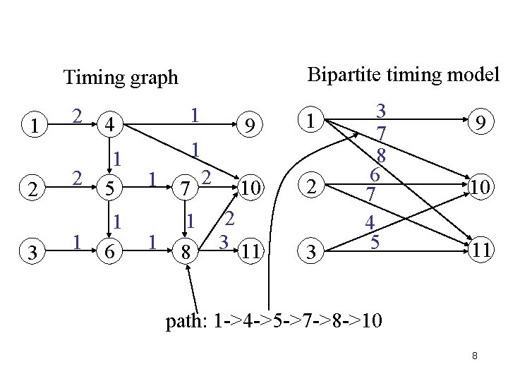
Bipartite timing model Timing graph 1 2 3 2 4 1 2 1 5 1 2 1 1 6 1 7 1 1 8 9 1 10 2 2 3 11 3 3 7 8 6 7 4 5 9 10 11 path: 1 ->4 ->5 ->7 ->8 ->10 8

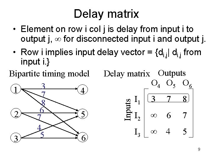
Delay matrix Inputs • Element on row i col j is delay from input i to output j, for disconnected input i and output j. • Row i implies input delay vector = {di, j| di, j from input i. } Delay matrix Outputs Bipartite timing model O 4 O 5 O 6 3 1 4 7 I 1 3 7 8 8 6 2 5 I 2 6 7 7 4 I 3 4 5 5 6 3 9

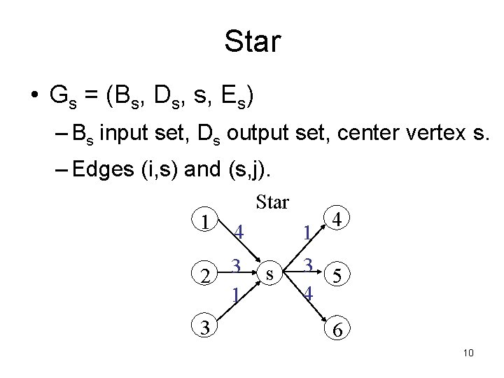
Star • Gs = (Bs, Ds, s, Es) – Bs input set, Ds output set, center vertex s. – Edges (i, s) and (s, j). 1 Star 4 2 3 1 s 4 3 5 4 6 10

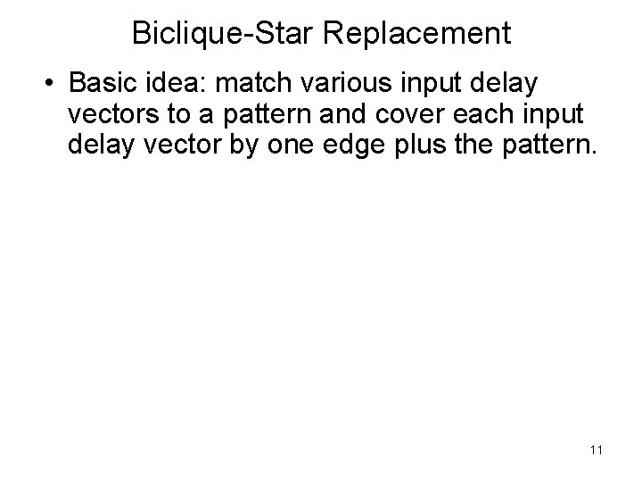
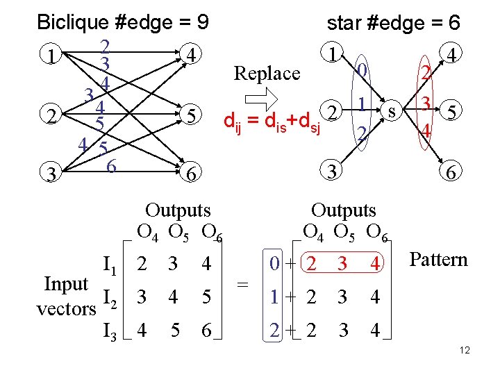
Biclique-Star Replacement • Basic idea: match various input delay vectors to a pattern and cover each input delay vector by one edge plus the pattern. 11

Biclique #edge = 9 2 4 1 3 Replace 4 3 4 5 dij = dis+dsj 2 5 4 5 6 6 3 Outputs O 4 O 5 O 6 I 1 2 3 4 Input I 2 3 4 5 vectors I 3 4 5 6 star #edge = 6 1 4 0 2 3 1 s 5 2 4 2 3 6 Outputs O 4 O 5 O 6 = 0+ 2 3 4 1+ 2 3 4 2+ 2 Pattern 3 4 12

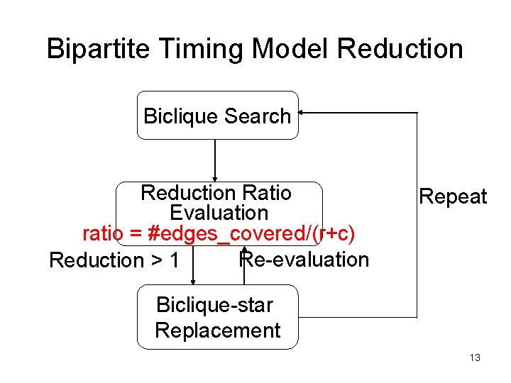
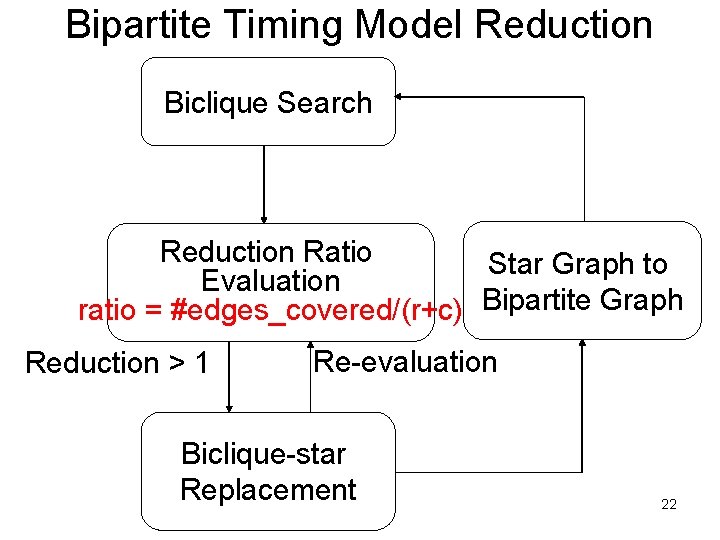
Bipartite Timing Model Reduction Biclique Search Reduction Ratio Evaluation ratio = #edges_covered/(r+c) Re-evaluation Reduction > 1 Repeat Biclique-star Replacement 13

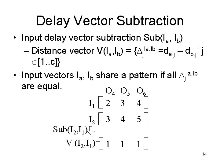
Delay Vector Subtraction • Input delay vector subtraction Sub(Ia, Ib) – Distance vector V(Ia, Ib) = { j. Ia, Ib =da, j – db, j| j [1. . c]} • Input vectors Ia, Ib share a pattern if all j. Ia, Ib are equal. O O O 4 5 6 I 1 2 3 4 I 2 3 4 5 Sub(I 2, I 1) V (I 2, I 1)= 1 14

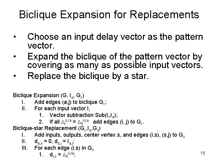
Biclique Expansion for Replacements • • • Choose an input delay vector as the pattern vector. Expand the biclique of the pattern vector by covering as many as possible input vectors. Replace the biclique by a star. Biclique Expansion (G, Ia, Gc) I. Add edges (a, j) to biclique Gc; II. For each input vector Ii 1. Vector subtraction Sub(Ii, Ia); 2. If all j. Ii, Ia = 0 Ii, Ia add edges (i, j) to Gc. Biclique-star Replacement (Gc, Ia, Gs) I. Add inputs, outputs, center vertex s, and edges (i, s), (s, j) to Gs II. da, s = 0, ds, j = Ia, j; III. For each edge (i, s) in Gs 1. di, s = 0 Ii, Ia; 15

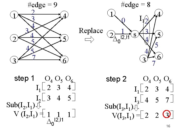
1 2 3 #edge = 9 2 4 3 4 5 5 45 7 6 step 1 O 4 O 5 O 6 I 1 2 3 4 I 2 3 4 5 Sub(I 2, I 1) V (I 2, I 1) = 1 1 1 0 I 2, I 1 #edge = 8 1 Replace 0 1 2 I 2, I 1 0 I 1 2 s 3 4 4 5 5 4 3 76 step 2 O 4 O 5 O 6 I 1 2 3 4 I 3 4 5 7 Sub(I 3, I 1) V(I 3, I 1) = 2 2 3 16

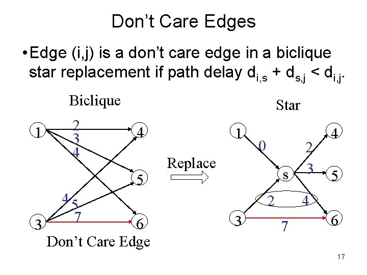
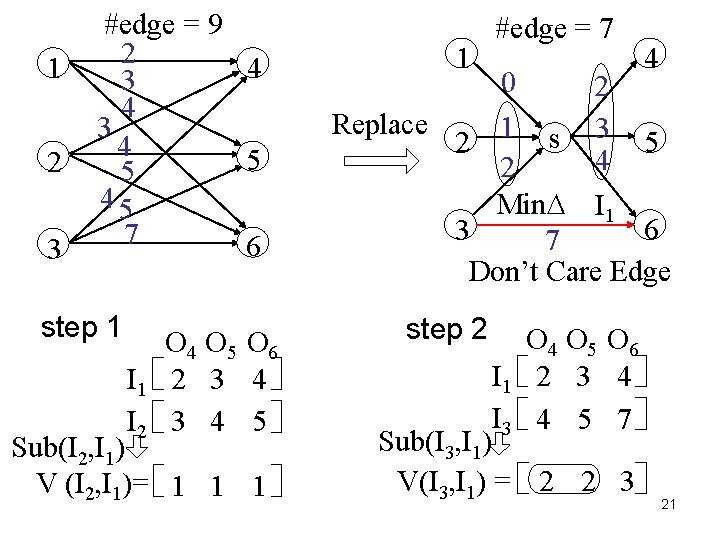
Don’t Care Edges • Edge (i, j) is a don’t care edge in a biclique star replacement if path delay di, s + ds, j < di, j. Biclique 1 2 3 4 Star 4 5 3 45 7 6 Don’t Care Edge 1 0 Replace s 2 3 4 5 4 7 6 17

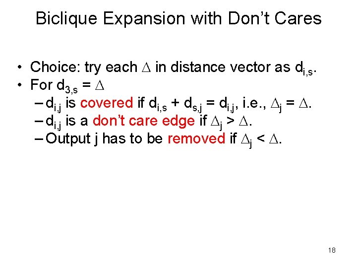
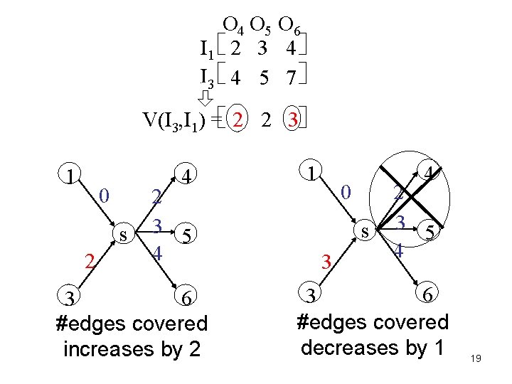
Biclique Expansion with Don’t Cares • Choice: try each in distance vector as di, s. • For d 3, s = – di, j is covered if di, s + ds, j = di, j, i. e. , j = . – di, j is a don’t care edge if j > . – Output j has to be removed if j < . 18

O 4 O 5 O 6 I 1 2 3 4 I 3 4 5 7 V(I 3, I 1) = 2 2 3 1 4 0 s 2 2 3 5 4 6 3 #edges covered increases by 2 1 4 0 s 3 2 3 5 4 6 3 #edges covered decreases by 1 19

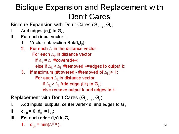
Biclique Expansion and Replacement with Don’t Cares Biclique Expansion with Don’t Cares (G, Ia, Gc) I. II. Add edges (a, j) to Gc; For each input vector Ii 1. Vector subtraction Sub(Ii, Ip); 2. For each j in the distance vector For each k in distance vector if k = j #covered++; else if k < j #removed +=edges to output k; 3. If maximum (#covered - #removed of j )> 1; For each k in distance vector if k j Add edge (i, k) to Gc; else remove output k and edges to k. Replacement with Don’t Cares (Gc, Ia, Gs) I. III. Add inputs, outputs, center vertex s, and edges to Gs da, s = 0, ds, j = Ia, j; For each edge (i, s) in Gs 1. di, s = min( Ii, Ia ). 20

1 2 3 #edge = 9 2 4 3 4 5 5 45 7 6 step 1 O 4 O 5 O 6 I 1 2 3 4 I 2 3 4 5 Sub(I 2, I 1) V (I 2, I 1)= 1 1 #edge = 7 4 0 2 Replace 1 s 3 5 2 4 2 Min I 1 6 3 7 Don’t Care Edge step 2 O 4 O 5 O 6 I 1 2 3 4 I 3 4 5 7 Sub(I 3, I 1) V(I 3, I 1) = 2 2 3 21

Bipartite Timing Model Reduction Biclique Search Reduction Ratio Star Graph to Evaluation ratio = #edges_covered/(r+c) Bipartite Graph Reduction > 1 Re-evaluation Biclique-star Replacement 22

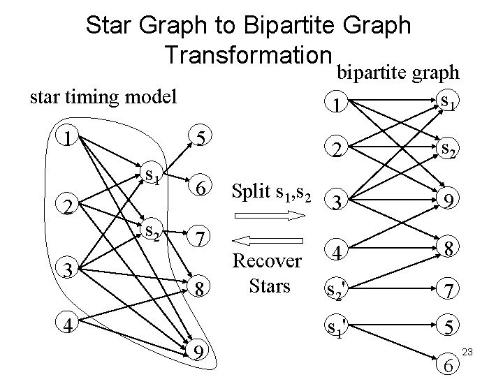
Star Graph to Bipartite Graph Transformation bipartite graph s 1 1 star timing model 1 5 s 1 2 3 s 2 6 7 8 4 9 Split s 1, s 2 Recover Stars 2 3 9 4 8 s 2' 7 s 1' 5 6 23

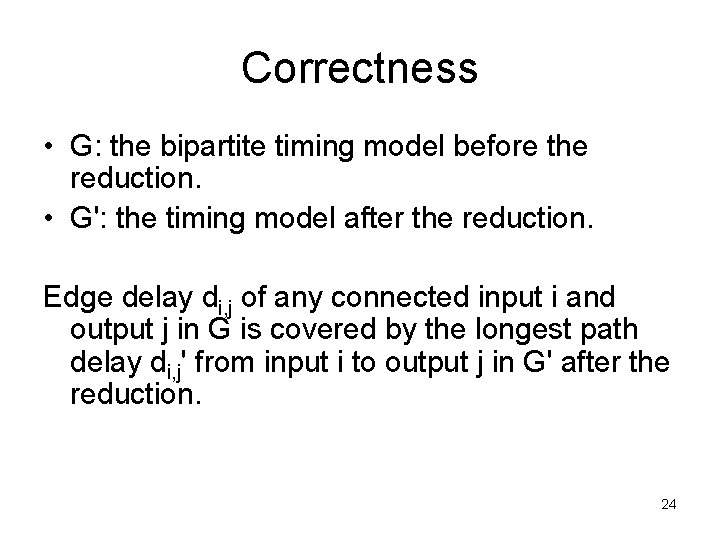
Correctness • G: the bipartite timing model before the reduction. • G': the timing model after the reduction. Edge delay di, j of any connected input i and output j in G is covered by the longest path delay di, j' from input i to output j in G' after the reduction. 24

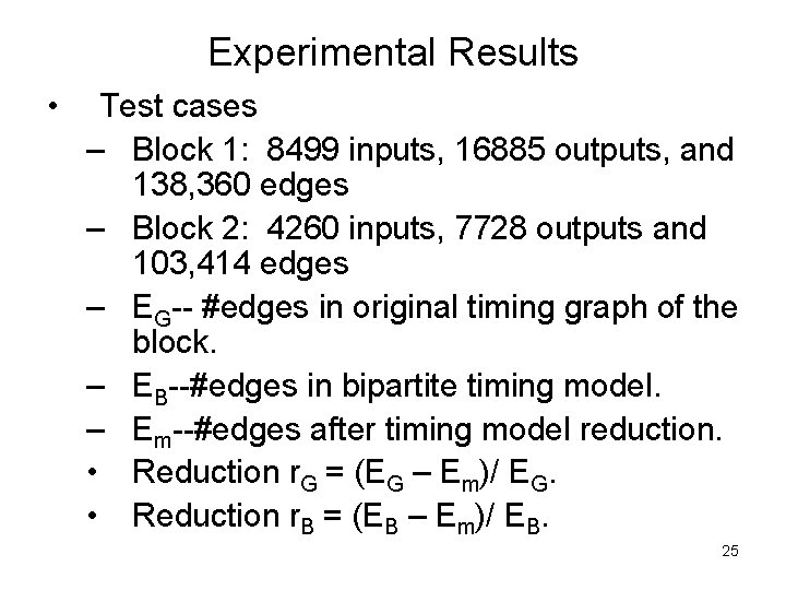
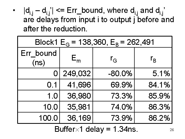
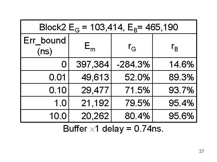
Experimental Results • Test cases – Block 1: 8499 inputs, 16885 outputs, and 138, 360 edges – Block 2: 4260 inputs, 7728 outputs and 103, 414 edges – EG-- #edges in original timing graph of the block. – EB--#edges in bipartite timing model. – Em--#edges after timing model reduction. • Reduction r. G = (EG – Em)/ EG. • Reduction r. B = (EB – Em)/ EB. 25

• |di, j – di, j’| <= Err_bound, where di, j and di, j’ are delays from input i to output j before and after the reduction. Block 1 EG = 138, 360, EB = 262, 491 Err_bound Em r. G r. B (ns) 0 249, 032 -80. 0% 5. 1% 0. 1 41, 696 69. 9% 84. 1% 1. 0 36, 980 73. 3% 85. 9% 10. 0 35, 981 74. 0% 86. 3% 100. 0 36, 169 73. 9% 86. 2% 26 Buffer 1 delay = 1. 34 ns.

Block 2 EG = 103, 414, EB= 465, 190 Err_bound Em r. G r. B (ns) 0 397, 384 -284. 3% 14. 6% 0. 01 49, 613 52. 0% 89. 3% 0. 10 29, 477 71. 5% 93. 7% 1. 0 21, 192 79. 5% 95. 4% 10. 0 20, 262 80. 4% 95. 6% Buffer 1 delay = 0. 74 ns. 27

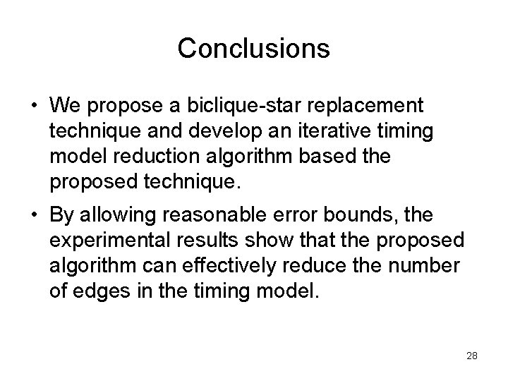
Conclusions • We propose a biclique-star replacement technique and develop an iterative timing model reduction algorithm based the proposed technique. • By allowing reasonable error bounds, the experimental results show that the proposed algorithm can effectively reduce the number of edges in the timing model. 28

Thanks! 29

References • C. W. Moon, H. ~Kriplani, and K. ~P. Belkhale, “Timing model extraction of hierarchical blocks by graph reduction”, in DAC’ 02, 152 -157. • C. Visweswariah and A. R. Conn, “Formulation of static circuit optimization with reduced size, degeneracy and redundancy by timing graph manipulation”, in ICCAD’ 99, 244 -251. • S. L. Hakimi and S. S. Yau. “Distance matrix of a graph and its realizability. ” Quart. Appl. Math. 22 (1964), 305– 317. • F. Chung, M. Garrett, R. Graham, and D. Shallcross. “Distance realization problems with applications to internet tomography. ” http: //www. math. ucsd. edu/˜fan. • T. Feder and A. Meyerson and R. Motwani and L. O' Callaghan and R. Panigrahy, “Representing graph metrics with fewest edges. ” in Proc. of Symp. on Theoretical Aspects of Computer Science (2003), 355 --366. 30