TimeAggregated Graphs Modeling Spatiotemporal Networks Prof Shashi Shekhar

Time-Aggregated Graphs. Modeling Spatio-temporal Networks Prof. Shashi Shekhar Department of Computer Science and Engineering University of Minnesota August 29, 2008 1

Selected Publications Time Aggregated Graphs n B. George, S. Shekhar, Time Aggregated Graphs for Modeling Spatio-temporal Networks-An Extended Abstract, Proceedings of Workshops (Co. Mo. GIS) at International Conference on Conceptual Modeling, (ER 2006) 2006. (Best Paper Award) n B. George, S. Kim, S. Shekhar, Spatio-temporal Network Databases and Routing Algorithms: A Summary of Results, Proceedings of International Symposium on Spatial and Temporal Databases (SSTD 07), July, 2007. n B. George, J. Kang, S. Shekhar, STSG: A Data Model for Representation and Knowledge Discovery in Sensor Data, Proceedings of Workshop on Knowledge Discovery from Sensor data at the International Conference on Knowledge Discovery and Data Mining (KDD) Conference, August 2007. (Best Paper Award). n B. George, S. Shekhar, Modeling Spatio-temporal Network Computations: A Summary of Results, Proceedings of Second International Conference on Geo. Spatial Semantics (Geo. S 2007), 2007. n B. George, S. Shekhar, Time Aggregated Graphs for Modeling Spatio-temporal Networks, Journal on Semantics of Data, Volume XI, Special issue of Selected papers from ER 2006, December 2007. n B. George, J. Kang, S. Shekhar, STSG: A Data Model for Representation and Knowledge Discovery in Sensor Data, Accepted for publication in Journal of Intelligent Data Analysis. n B. George, S. Shekhar, Routing Algorithms in Non-stationary Transportation Network, Proceedings of International Workshop on Computational Transportation Science, Dublin, Ireland, July, 2008. n B. George, S. Shekhar, S. Kim, Routing Algorithms in Spatio-temporal Databases, Transactions on Data and Knowledge Engineering (In submission). Evacuation Planning n Q Lu, B. George, S. Shekhar, Capacity Constrained Routing Algorithms for Evacuation Planning: A Summary of Results, Proceedings of International Symposium on Spatial and Temporal Databases (SSTD 05), August, 2005. n S. Kim, B. George, S. Shekhar, Evacuation Route Planning: Scalable Algorithms, Proceedings of ACM International Symposium on Advances in Geographic Information Systems (ACMGIS 07), November, 2007. n Q Lu, B. George, S. Shekhar, Capacity Constrained Routing Algorithms for Evacuation Planning, International Journal of Semantic Computing, Volume 1, No. 2, June 2007. 2

Outline q Introduction q q q Motivation Problem Statement Related Work Contributions q Representation q Routing Algorithms Conclusion and Future Work 3

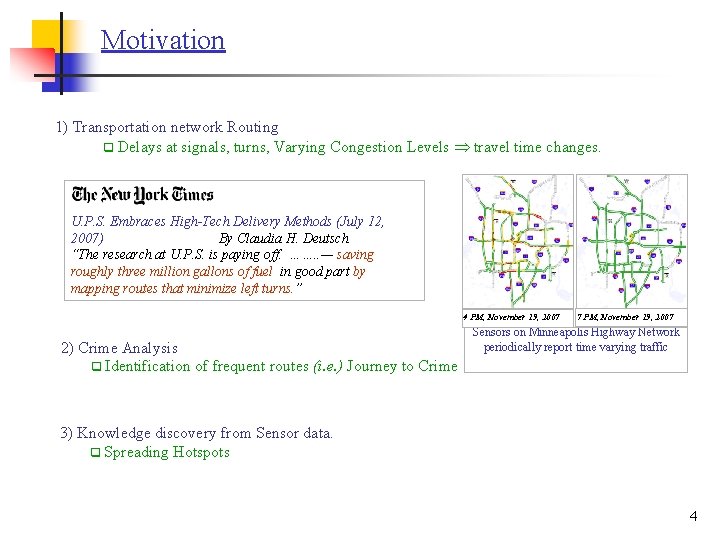
Motivation 1) Transportation network Routing q Delays at signals, turns, Varying Congestion Levels travel time changes. U. P. S. Embraces High-Tech Delivery Methods (July 12, 2007) By Claudia H. Deutsch “The research at U. P. S. is paying off. ……. . — saving roughly three million gallons of fuel in good part by mapping routes that minimize left turns. ” 9 PM, November 19, 2007 4 PM, November 19, 2007 2) Crime Analysis q Identification of frequent routes (i. e. ) Journey to Crime 7 PM, November 19, 2007 Sensors on Minneapolis Highway Network periodically report time varying traffic 3) Knowledge discovery from Sensor data. q Spreading Hotspots 4

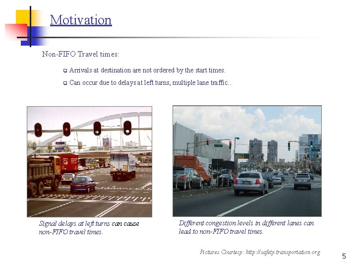
Motivation Non-FIFO Travel times: q Arrivals at destination are not ordered by the start times. q Can occur due to delays at left turns, multiple lane traffic. . Signal delays at left turns can cause non-FIFO travel times. Different congestion levels in different lanes can lead to non-FIFO travel times. Pictures Courtesy: http: //safety. transportation. org 5

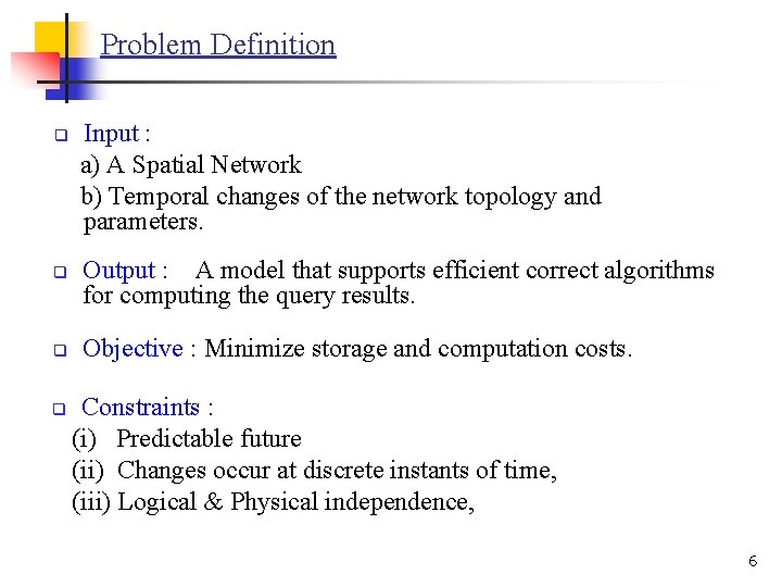
Problem Definition q q Input : a) A Spatial Network b) Temporal changes of the network topology and parameters. Output : A model that supports efficient correct algorithms for computing the query results. Objective : Minimize storage and computation costs. Constraints : (i) Predictable future (ii) Changes occur at discrete instants of time, (iii) Logical & Physical independence, 6

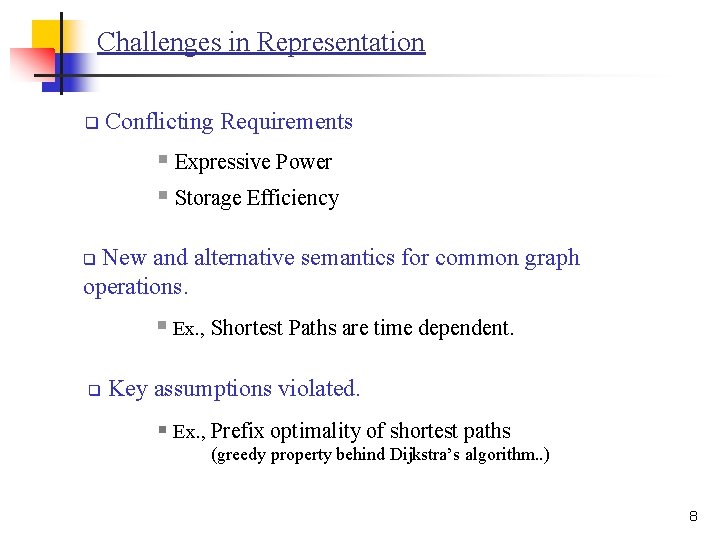
Challenges in Representation q Conflicting Requirements § Expressive Power § Storage Efficiency New and alternative semantics for common graph operations. q § Ex. , Shortest Paths are time dependent. q Key assumptions violated. § Ex. , Prefix optimality of shortest paths (greedy property behind Dijkstra’s algorithm. . ) 8

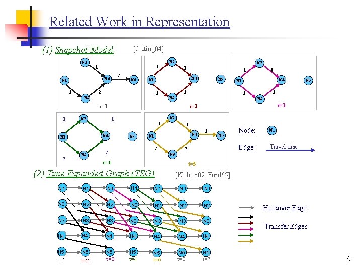
Related Work in Representation (1) Snapshot Model N 2 1 1 2 N 4 N 1 2 [Guting 04] N 5 N 2 1 N 4 N 1 2 2 N 3 N 2 2 2 N 3 N 4 N 1 N 5 2 2 N 3 t=2 N 2 1 N 4 N 1 N 5 N 3 t=1 1 1 N 5 1 N 4 N 1 N 5 2 2 Node: N. . Edge: Travel time N 3 t=4 t=5 (2) Time Expanded Graph (TEG) [Kohler 02, Ford 65] N 1 N 1 N 2 N 2 N 3 N 3 N 4 N 4 N 5 t=1 t=2 N 5 t=3 N 5 t=4 N 5 t=5 N 5 t=6 N 5 t=7 Holdover Edge Transfer Edges 9

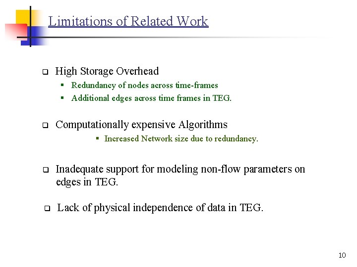
Limitations of Related Work q High Storage Overhead § Redundancy of nodes across time-frames § Additional edges across time frames in TEG. q Computationally expensive Algorithms § Increased Network size due to redundancy. q Inadequate support for modeling non-flow parameters on edges in TEG. q Lack of physical independence of data in TEG. 10

Outline q Introduction q q Motivation Problem Statement Related Work Contributions q Representation �Time Aggregated Graph (TAG) q Case Studies �Routing Algorithms q Conclusion and Future Work 11

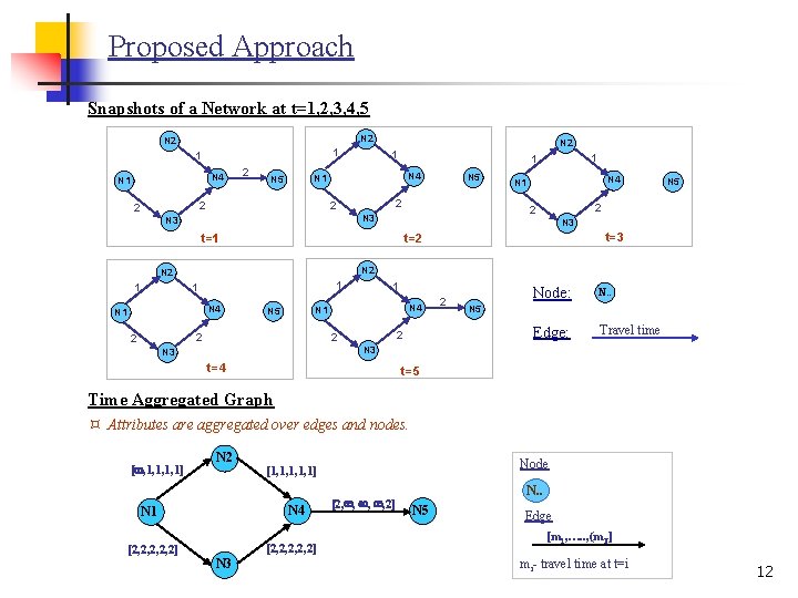
Proposed Approach Snapshots of a Network at t=1, 2, 3, 4, 5 N 2 1 1 N 4 N 1 2 N 4 N 5 2 N 3 t=2 t=1 N 2 1 1 N 4 N 1 N 5 2 2 N 4 N 1 2 N 3 1 N 5 2 2 1 1 N 5 2 2 N 2 1 2 Node: N. . Edge: Travel time N 5 N 3 t=4 t=5 Time Aggregated Graph ³ Attributes are aggregated over edges and nodes. [ , 1, 1] N 2 N 4 N 1 [2, 2, 2] N 3 Node [1, 1, 1] [2, , , , 2] N. . N 5 Edge [m 1, …. . , (m. T] mi- travel time at t=i 12

Time Aggregated Graph TAG = (N, E, T, [nw 1…nw. T ], [ew 1, . . , ew. T ] | nwi : N RT, ewi : E RT N : Set of nodes E : Set of edges T : Length of time interval nwi: Time dependent attribute on nodes for time instant i. ewi: Time dependent attribute on edges for time instant i. On edge N 4 -N 5 * [2, ∞, ∞, ∞, 2] is a time series of attribute; [ , 1, 1] N 2 [1, 1, 1] N 4 N 1 [2, , , , 2] N 5 * At t=1, the edge has an attribute value of 2. * At t=2, the ‘∞’ can indicate the absence of connectivity between the nodes at t=2. [2, 2, 2] N 3 13

Performance Evaluation: Dataset Minneapolis CBD [1/2, 1, 2, 3 miles radii] Dataset # Nodes # Edges 1. (MPLS -1/2) 111 287 2. (MPLS -1 mi) 277 674 3. (MPLS - 2 mi) 562 1443 4. (MPLS - 3 mi) 786 2106 Road data Mn/DOT basemap for MPLS CBD. 14

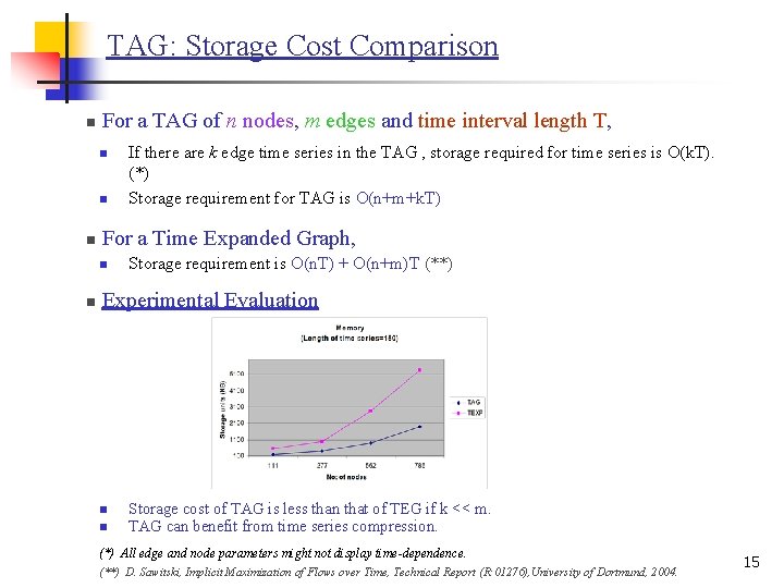
TAG: Storage Cost Comparison n For a TAG of n nodes, m edges and time interval length T, n n n For a Time Expanded Graph, n n If there are k edge time series in the TAG , storage required for time series is O(k. T). (*) Storage requirement for TAG is O(n+m+k. T) Storage requirement is O(n. T) + O(n+m)T (**) Experimental Evaluation n n Storage cost of TAG is less than that of TEG if k << m. TAG can benefit from time series compression. (*) All edge and node parameters might not display time-dependence. (**) D. Sawitski, Implicit Maximization of Flows over Time, Technical Report (R: 01276), University of Dortmund, 2004. 15

Outline q Introduction q q Motivation Problem Statement Related Work Contributions q Representation �Time Aggregated Graph (TAG) q q Routing Algorithms Conclusion and Future Work 16

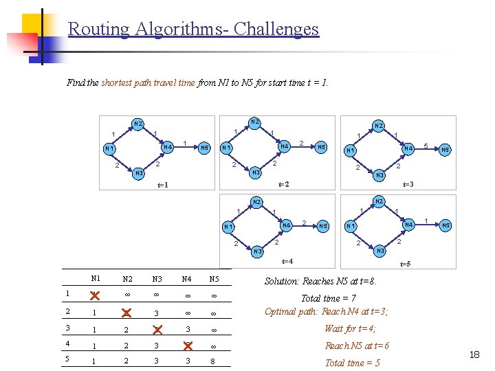
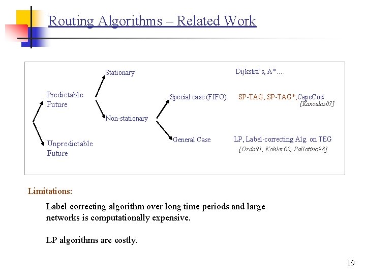
Routing Algorithms- Challenges q Violation of optimal prefix property q Not all optimal paths show optimal prefix property. q New and Alternate semantics q Termination of the algorithm: an infinite non-negative cycle over time 17

Routing Algorithms- Challenges Find the shortest path travel time from N 1 to N 5 for start time t = 1. N 2 1 1 1 N 4 N 1 1 2 N 5 N 4 N 1 2 2 t=3 t=2 N 2 1 1 N 4 N 1 2 2 N 5 N 3 t=1 1 5 2 2 N 3 1 1 N 4 N 1 N 5 2 2 N 2 1 2 N 5 1 N 4 N 1 1 N 5 2 2 N 3 t=4 t=5 N 1 N 2 N 3 N 4 N 5 Solution: Reaches N 5 at t=8. 1 1 ∞ ∞ 2 1 2 3 ∞ ∞ Total time = 7 Optimal path: Reach N 4 at t=3; 3 1 2 3 3 ∞ Wait for t=4; 4 1 2 3 3 ∞ Reach N 5 at t=6 5 1 2 3 3 8 Total time = 5 18

Routing Algorithms – Related Work Dijkstra’s, A*…. Stationary Predictable Future Special case (FIFO) SP-TAG, SP-TAG*, Cape. Cod [Kanoulas 07] Non-stationary Unpredictable Future General Case LP, Label-correcting Alg. on TEG [Orda 91, Kohler 02, Pallotino 98] Limitations: Label correcting algorithm over long time periods and large networks is computationally expensive. LP algorithms are costly. 19

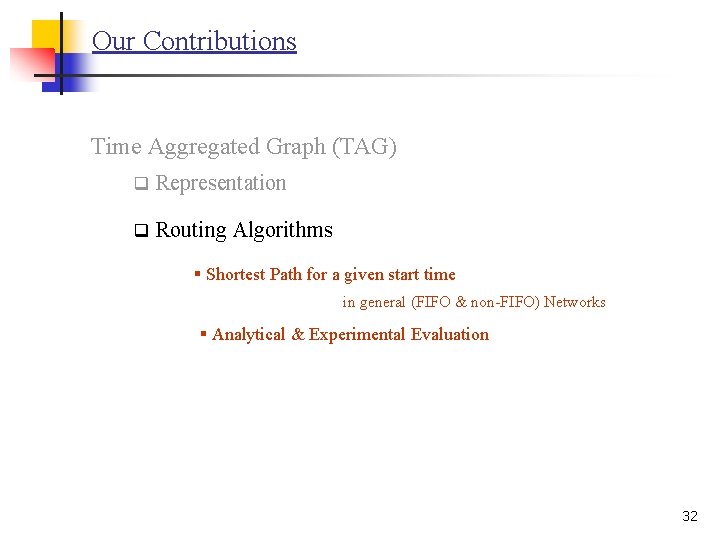
Our Contributions Time Aggregated Graph (TAG) q Representation q Routing Algorithms § Shortest Path for a given start time in general (FIFO & non-FIFO) Networks § Analytical & Experimental Evaluation 32

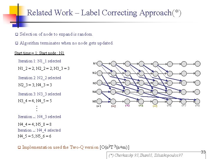
Related Work – Label Correcting Approach(*) q Selection of node to expand is random. q Algorithm terminates when no node gets updated. Start time = 1; Start node : N 1 Iteration 1: N 1_1 selected N 1_2 = 2; N 2_2 = 2; N 3_3 = 3 N 2 Iteration 2: N 2_2 selected N 2_3 = 3; N 4_3 = 3 Iteration 3: N 3_3 selected N 3_4 = 4; N 4_5 = 5 . . . N 3 N 4 N 5 t=1 t=2 t=3 t=4 t=5 t=6 t=7 t=8 Iteration. . : N 4_3 selected N 4_4 = 4; N 5_8 = 8 Iteration. . : N 4_4 selected N 4_5 = 5; N 5_6 = 6 q Implementation used the Two-Q version [O(n 2 T 3(n+m)] (*) Cherkassky 93, Zhan 01, Ziliaskopoulos 97 33

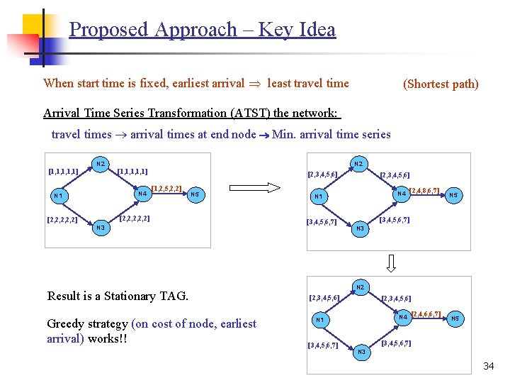
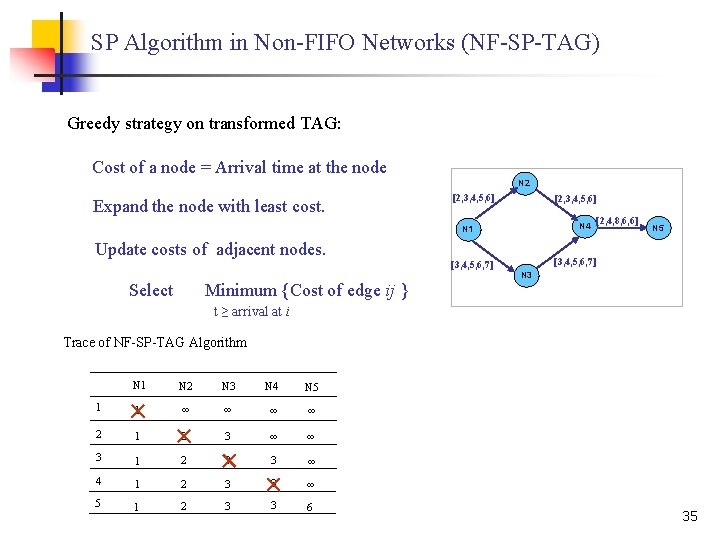
Proposed Approach – Key Idea When start time is fixed, earliest arrival least travel time (Shortest path) Arrival Time Series Transformation (ATST) the network: travel times arrival times at end node Min. arrival time series [1, 1, 1] N 2 [1, 1, 1] N 4 N 1 [2, 3, 4, 5, 6] [1, 2, 5, 2, 2] N 5 [2, 2, 2] N 3 Result is a Stationary TAG. Greedy strategy (on cost of node, earliest arrival) works!! [2, 3, 4, 5, 6] N 4 [2, 4, 8, 6, 7] N 1 [3, 4, 5, 6, 7] N 5 [3, 4, 5, 6, 7] N 3 N 2 [2, 3, 4, 5, 6] N 4 [2, 4, 6, 6, 7] N 1 [3, 4, 5, 6, 7] N 5 [3, 4, 5, 6, 7] N 3 34

SP Algorithm in Non-FIFO Networks (NF-SP-TAG) Greedy strategy on transformed TAG: Cost of a node = Arrival time at the node N 2 Expand the node with least cost. [2, 3, 4, 5, 6] N 4 [2, 4, 8, 6, 6] N 1 Update costs of adjacent nodes. Select [3, 4, 5, 6, 7] N 5 [3, 4, 5, 6, 7] N 3 Minimum {Cost of edge ij } t ≥ arrival at i Trace of NF-SP-TAG Algorithm N 1 N 2 N 3 N 4 N 5 1 1 ∞ ∞ 2 1 2 3 ∞ ∞ 3 1 2 3 3 ∞ 4 1 2 3 3 ∞ 5 1 2 3 3 6 35

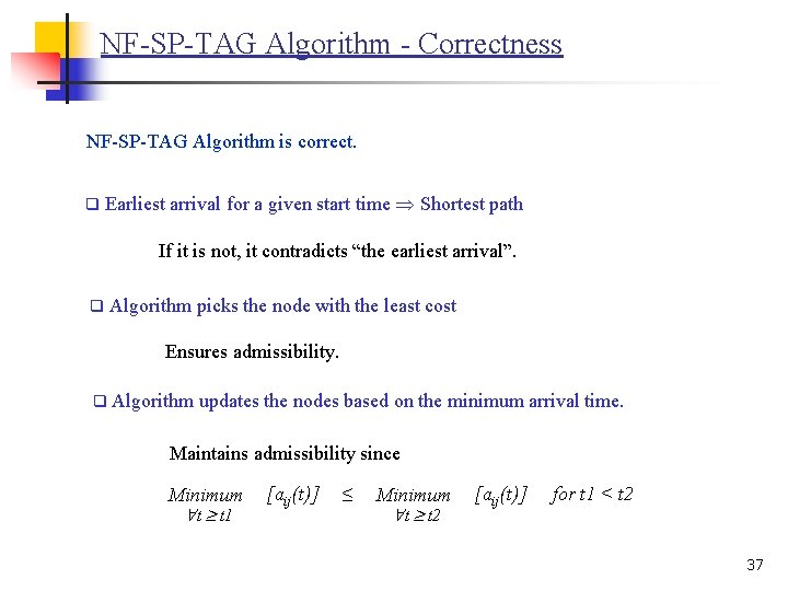
NF-SP-TAG Algorithm- Pseudocode n n Pre-process the network. Initialize c[s] = t_start; v ( s), c[v] = ∞. Insert s in the priority queue Q. while Q is not empty do u = extract_min(Q); close u (C = C {u}) for each node v adjacent to u do { t = min_arrival((u, v), c[u]); if t + u, v(t) < c[v] = t + u, v(t) parent[v] = u insert v in Q if it is not in Q; } Update Q. 36

NF-SP-TAG Algorithm - Correctness NF-SP-TAG Algorithm is correct. q Earliest arrival for a given start time Shortest path If it is not, it contradicts “the earliest arrival”. q Algorithm picks the node with the least cost Ensures admissibility. q Algorithm updates the nodes based on the minimum arrival time. Maintains admissibility since Minimum t t 1 [aij(t)] ≤ Minimum t t 2 [aij(t)] for t 1 < t 2 37

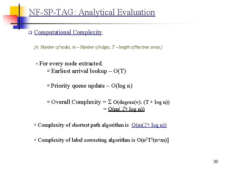
NF-SP-TAG: Analytical Evaluation q Computational Complexity [n: Number of nodes, m – Number of edges, T – length of the time series] ú For every node extracted, ú Earliest arrival lookup – O(T) ú Priority queue update – O(log n) ú Overall Complexity = O(degree(v). (T + log n)) = O(m( T+ log n)) ú Complexity of shortest path algorithm is O(m(T+ log n)) ú Complexity of label correcting algorithm is O(n 2 T 3(n+m)] 38

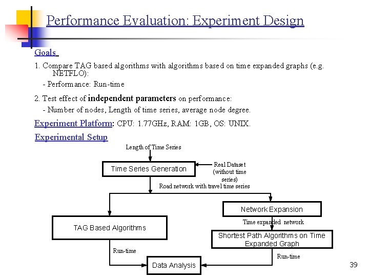
Performance Evaluation: Experiment Design Goals 1. Compare TAG based algorithms with algorithms based on time expanded graphs (e. g. NETFLO): - Performance: Run-time 2. Test effect of independent parameters on performance: - Number of nodes, Length of time series, average node degree. Experiment Platform: CPU: 1. 77 GHz, RAM: 1 GB, OS: UNIX. Experimental Setup Length of Time Series Real Dataset (without time series) Road network with travel time series Time Series Generation Network Expansion Time expanded network TAG Based Algorithms Shortest Path Algorithms on Time Expanded Graph Run-time Data Analysis 39

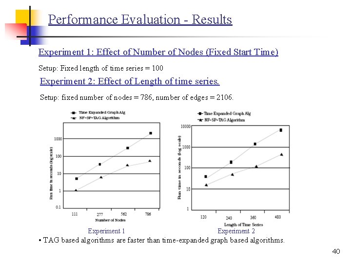
Performance Evaluation - Results Experiment 1: Effect of Number of Nodes (Fixed Start Time) Setup: Fixed length of time series = 100 Experiment 2: Effect of Length of time series. Setup: fixed number of nodes = 786, number of edges = 2106. Experiment 1 Experiment 2 • TAG based algorithms are faster than time-expanded graph based algorithms. 40

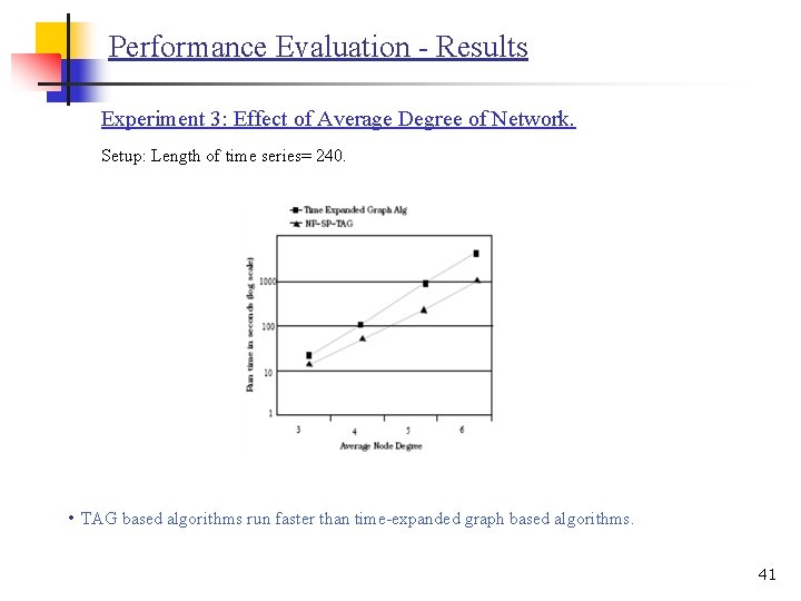
Performance Evaluation - Results Experiment 3: Effect of Average Degree of Network. Setup: Length of time series= 240. • TAG based algorithms run faster than time-expanded graph based algorithms. 41

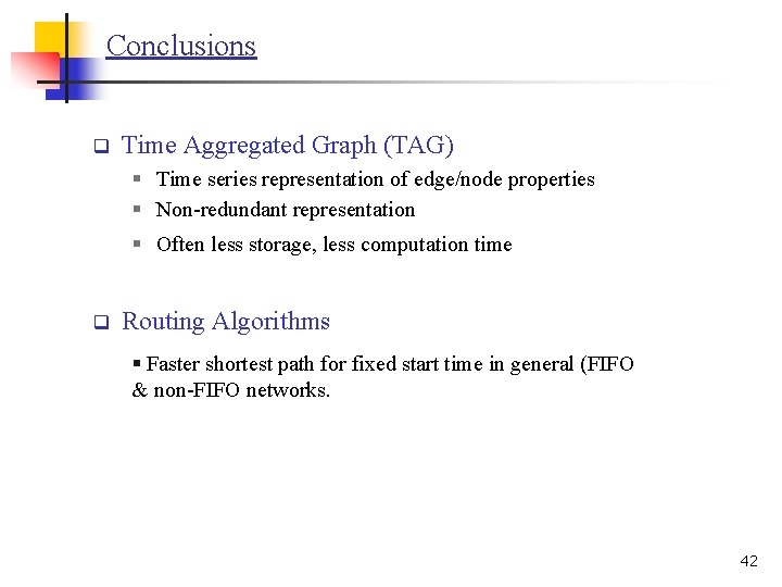
Conclusions q Time Aggregated Graph (TAG) § Time series representation of edge/node properties § Non-redundant representation § Often less storage, less computation time q Routing Algorithms § Faster shortest path for fixed start time in general (FIFO & non-FIFO networks. 42

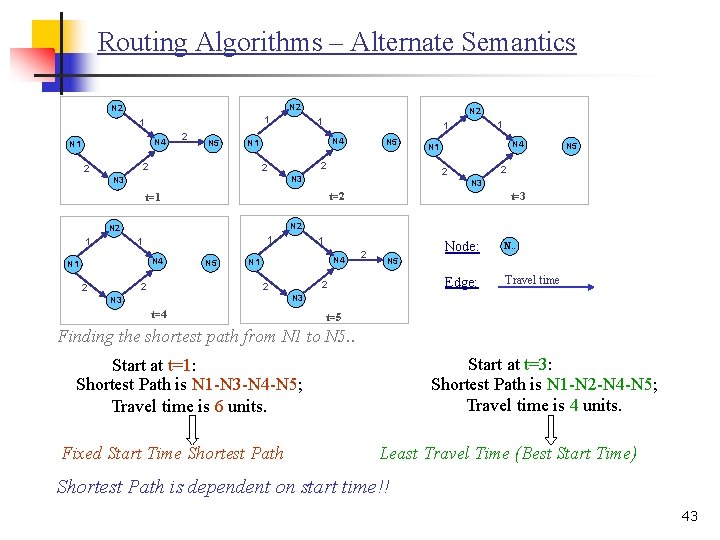
Routing Algorithms – Alternate Semantics N 2 1 1 N 4 N 1 2 N 5 2 N 3 t=2 N 2 1 1 N 4 N 1 N 5 1 N 4 N 1 2 Node: N. . Edge: Travel time N 5 2 2 N 4 N 1 2 N 3 t=1 1 N 5 2 2 N 3 1 1 N 4 N 1 2 2 N 2 1 N 3 t=4 t=5 Finding the shortest path from N 1 to N 5. . Start at t=3: Shortest Path is N 1 -N 2 -N 4 -N 5; Travel time is 4 units. Start at t=1: Shortest Path is N 1 -N 3 -N 4 -N 5; Travel time is 6 units. Fixed Start Time Shortest Path Least Travel Time (Best Start Time) Shortest Path is dependent on start time!! 43

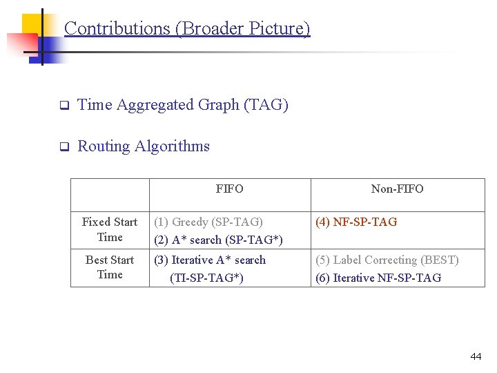
Contributions (Broader Picture) q Time Aggregated Graph (TAG) q Routing Algorithms FIFO Non-FIFO Fixed Start Time (1) Greedy (SP-TAG) (2) A* search (SP-TAG*) (4) NF-SP-TAG Best Start Time (3) Iterative A* search (TI-SP-TAG*) (5) Label Correcting (BEST) (6) Iterative NF-SP-TAG 44

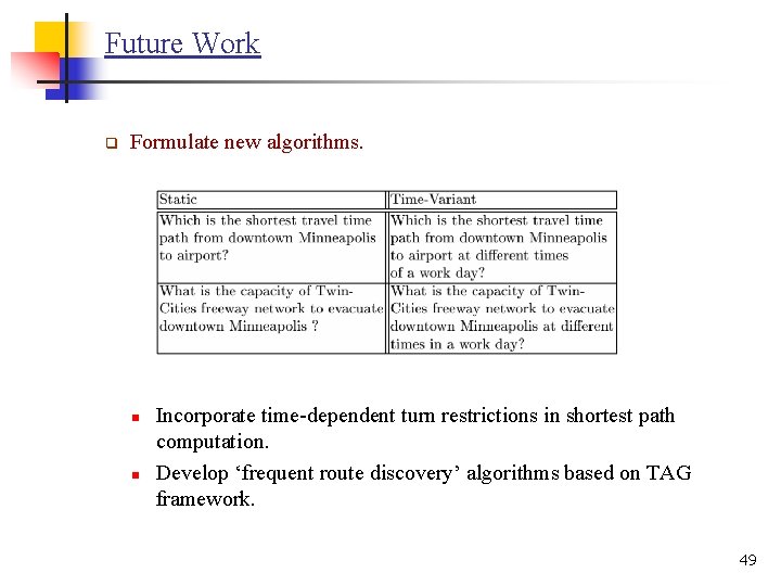
Future Work q Formulate new algorithms. n n Incorporate time-dependent turn restrictions in shortest path computation. Develop ‘frequent route discovery’ algorithms based on TAG framework. 49

Thank you. 50