Time stepping schemes for atmospheric modelling by Michail

Time stepping schemes for atmospheric modelling by Michail Diamantakis (room 2107; ext. 2402) michail. diamantakis@ecmwf. int Time stepping schemes for atmospheric modelling Slide 1 ECMWF

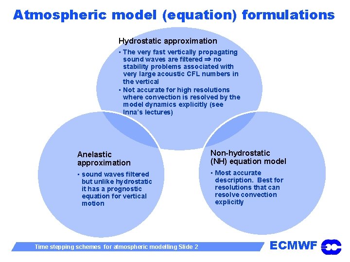
Atmospheric model (equation) formulations Hydrostatic approximation • The very fast vertically propagating sound waves are filtered ⇒ no stability problems associated with very large acoustic CFL numbers in the vertical • Not accurate for high resolutions where convection is resolved by the model dynamics explicitly (see Inna’s lectures) Anelastic approximation Non-hydrostatic (NH) equation model • sound waves filtered but unlike hydrostatic it has a prognostic equation for vertical motion • Most accurate description. Best for resolutions that can resolve convection explicitly Time stepping schemes for atmospheric modelling Slide 2 ECMWF

What motions time-stepping should resolve? t Rossby waves & slow gravity waves must be resolved and transported accurately – important for good weather predictions t Fast acoustic waves carry little energy and are not important for weather but for stability reasons they may limit severely timestep q To avoid such timestep restrictions, ideally an unconditionally stable numerical scheme is needed which may damp acoustic waves while is not damping other meteorologically important waves t Very high orders of accuracy in time-stepping are not necessary: q In any model, errors from other model components such as parametrizations are usually large enough to make use of very high integration order not a practical option. Often order 2 -3 is sufficient (also depends on space discretization order) Time stepping schemes for atmospheric modelling Slide 3 ECMWF

Scalability: an important requirement t CPU clock-speeds have stagnated - even decreasing (to reduce energy consumption) t More parallelism is the only way to achieve same time-to-solution when model resolution increases t Operational NWP solvers must scale well on very large number of cores ( >O(104) ) t Regular lat/lon grid global models are not practical at 1 km scales: t If explicit timestepping is used: meridian convergence at poles ⇒ extremely high resolution which limits severely ∆t t If implicit: grid anisotropy near poles leads to poor convergence of elliptic solvers + high communication cost t Global spectral transform models with reduced Gaussian grids at 1 km: may not scale well mainly due to high communication cost Time stepping schemes for atmospheric modelling Slide 4 ECMWF

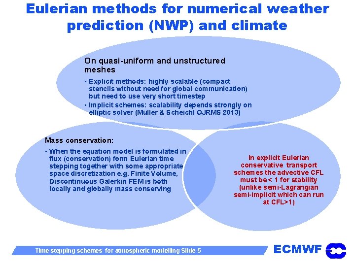
Eulerian methods for numerical weather prediction (NWP) and climate On quasi-uniform and unstructured meshes • Explicit methods: highly scalable (compact stencils without need for global communication) but need to use very short timestep • Implicit schemes: scalability depends strongly on elliptic solver (Müller & Scheichl QJRMS 2013) Mass conservation: • When the equation model is formulated in flux (conservation) form Eulerian time stepping together with some appropriate space discretization e. g. Finite Volume, Discontinuous Galerkin FEM is both locally and globally mass conserving Time stepping schemes for atmospheric modelling Slide 5 In explicit Eulerian conservative transport schemes the advective CFL must be < 1 for stability (unlike semi-Lagrangian semi-implicit which can run at CFL>1) ECMWF

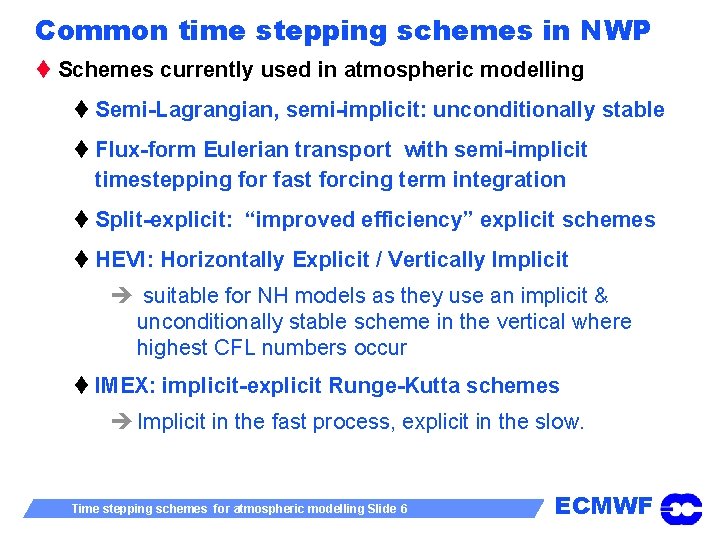
Common time stepping schemes in NWP t Schemes currently used in atmospheric modelling t Semi-Lagrangian, semi-implicit: unconditionally stable t Flux-form Eulerian transport with semi-implicit timestepping for fast forcing term integration t Split-explicit: “improved efficiency” explicit schemes t HEVI: Horizontally Explicit / Vertically Implicit è suitable for NH models as they use an implicit & unconditionally stable scheme in the vertical where highest CFL numbers occur t IMEX: implicit-explicit Runge-Kutta schemes è Implicit in the fast process, explicit in the slow. Time stepping schemes for atmospheric modelling Slide 6 ECMWF

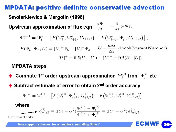
MPDATA: positive definite conservative advection Smolarkiewicz & Margolin (1998) Upstream approximation of flux eqn: MPDATA steps t Compute 1 st order upstream approximation from etc t Subtract estimate of error to obtain 2 nd order accuracy where Pseudo-velocity Time stepping schemes for atmospheric modelling Slide 7 ECMWF

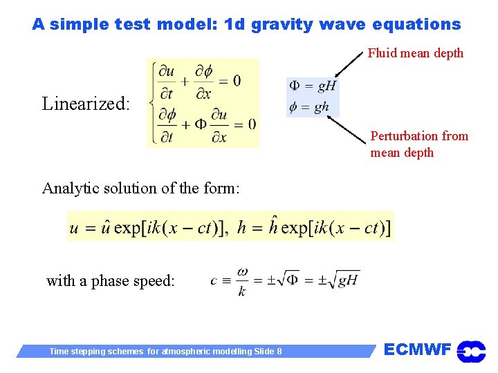
A simple test model: 1 d gravity wave equations Fluid mean depth Linearized: Perturbation from mean depth Analytic solution of the form: with a phase speed: Time stepping schemes for atmospheric modelling Slide 8 ECMWF

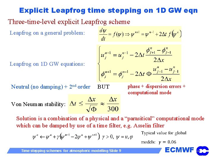
Explicit Leapfrog time stepping on 1 D GW eqn Three-time-level explicit Leapfrog scheme Leapfrog on a general problem: Leapfrog on 1 D GW equations: Neutral (no damping) + 2 nd order BUT phase + dispersion errors + computational mode Von Neuman stability: Solution is a combination of a physical and a “parasitical” computational mode which can be damped by use of a time filter, e. g. Asselin filter Time stepping schemes for atmospheric modelling Slide 9 ECMWF

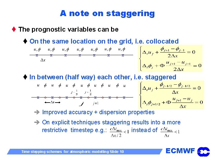
A note on staggering t The prognostic variables can be t On the same location on the grid, i. e. collocated x x t In between (half way) each other, i. e. staggered x o x o x è Improved accuracy + dispersion properties è On explicit techniques staggering results into a more restrictive timestep e. g. : instead of Time stepping schemes for atmospheric modelling Slide 10 ECMWF

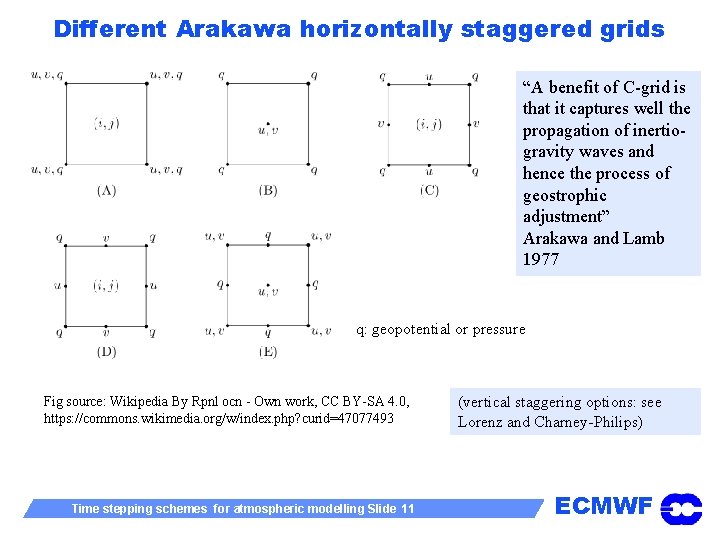
Different Arakawa horizontally staggered grids “A benefit of C-grid is that it captures well the propagation of inertiogravity waves and hence the process of geostrophic adjustment” Arakawa and Lamb 1977 q: geopotential or pressure Fig source: Wikipedia By Rpnl ocn - Own work, CC BY-SA 4. 0, https: //commons. wikimedia. org/w/index. php? curid=47077493 Time stepping schemes for atmospheric modelling Slide 11 (vertical staggering options: see Lorenz and Charney-Philips) ECMWF

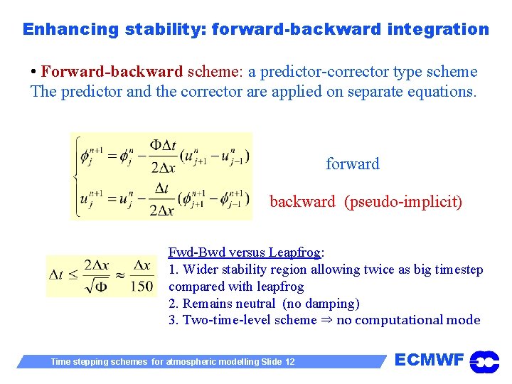
Enhancing stability: forward-backward integration • Forward-backward scheme: a predictor-corrector type scheme The predictor and the corrector are applied on separate equations. forward backward (pseudo-implicit) Fwd-Bwd versus Leapfrog: 1. Wider stability region allowing twice as big timestep compared with leapfrog 2. Remains neutral (no damping) 3. Two-time-level scheme ⇒ no computational mode Time stepping schemes for atmospheric modelling Slide 12 ECMWF

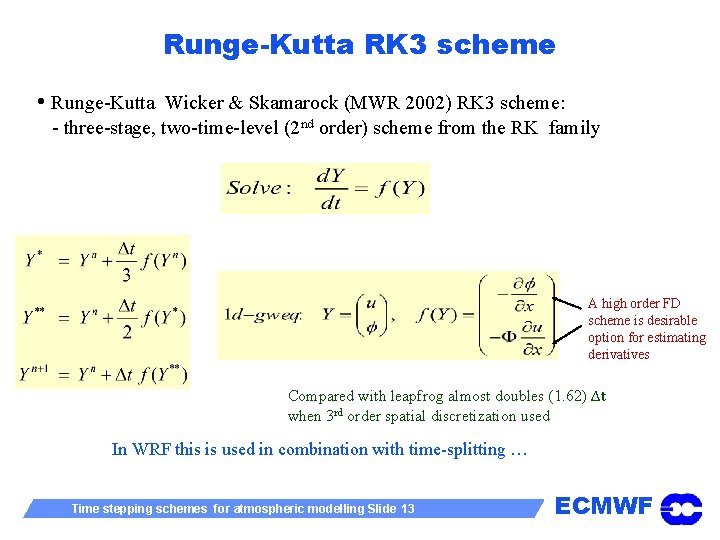
Runge-Kutta RK 3 scheme • Runge-Kutta Wicker & Skamarock (MWR 2002) RK 3 scheme: - three-stage, two-time-level (2 nd order) scheme from the RK family A high order FD scheme is desirable option for estimating derivatives Compared with leapfrog almost doubles (1. 62) Δt when 3 rd order spatial discretization used In WRF this is used in combination with time-splitting … Time stepping schemes for atmospheric modelling Slide 13 ECMWF

Splitting the time integration: the motivation t In an atmospheric model we have motions with multiple time-scales: fast and slow changing processes co-exist t Explicit techniques are only conditionally stable and that imposes use of small timesteps for fast propagating waves or when the solution changes rapidly in general t If ∆t is the longest permissible timestep for integrating the slow process then ∆t will be too long for stable integration of the fast process t A solution is to split the integration: è integrate slow changing process with ∆t è integrate fast changing process with a fraction of it i. e. ∆t/n Time stepping schemes for atmospheric modelling Slide 14 ECMWF

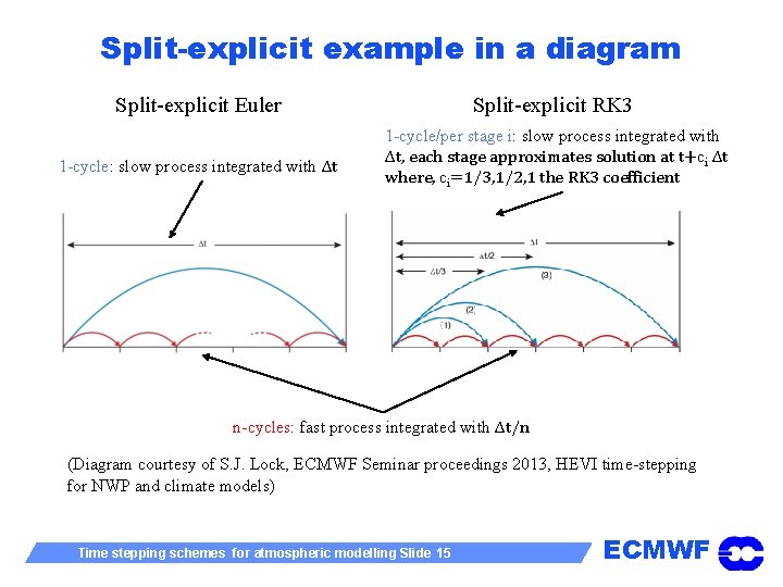
Split-explicit example in a diagram Split-explicit Euler Split-explicit RK 3 1 -cycle: slow process integrated with Δt 1 -cycle/per stage i: slow process integrated with Δt, each stage approximates solution at t+ci Δt where, ci=1/3, 1/2, 1 the RK 3 coefficient n-cycles: fast process integrated with Δt/n (Diagram courtesy of S. J. Lock, ECMWF Seminar proceedings 2013, HEVI time-stepping for NWP and climate models) Time stepping schemes for atmospheric modelling Slide 15 ECMWF

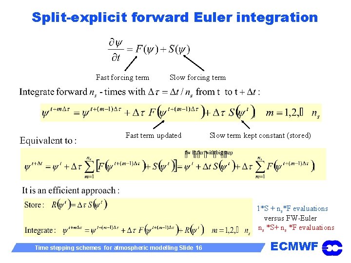
Split-explicit forward Euler integration Fast forcing term Slow forcing term Fast term updated Slow term kept constant (stored) 1*S + ns*F evaluations versus FW-Euler ns *S+ ns *F evaluations Time stepping schemes for atmospheric modelling Slide 16 ECMWF

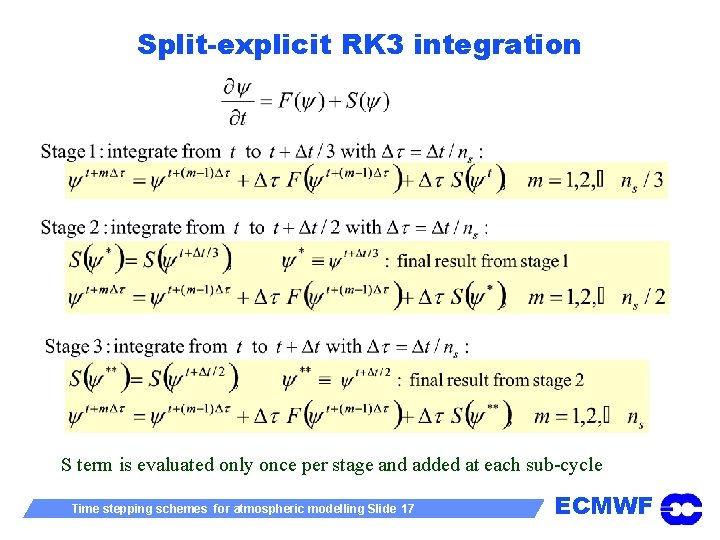
Split-explicit RK 3 integration S term is evaluated only once per stage and added at each sub-cycle Time stepping schemes for atmospheric modelling Slide 17 ECMWF

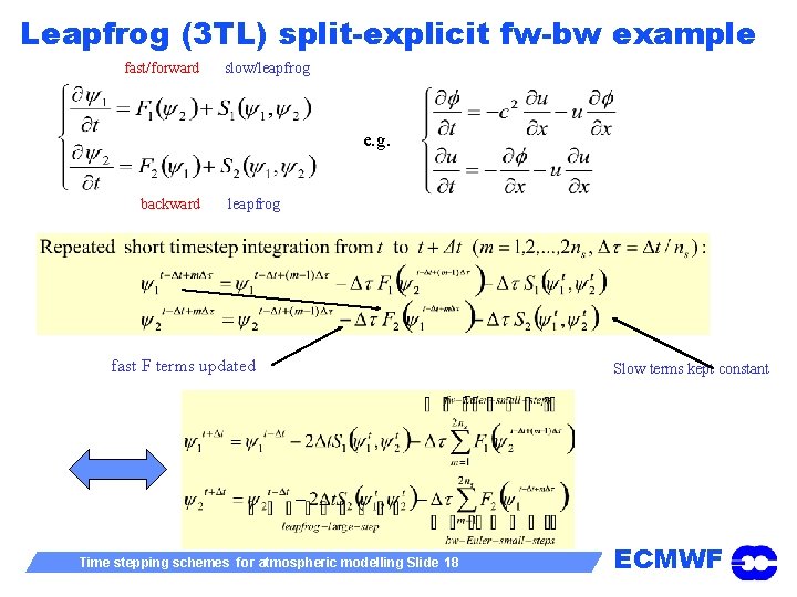
Leapfrog (3 TL) split-explicit fw-bw example fast/forward slow/leapfrog e. g. backward leapfrog fast F terms updated Time stepping schemes for atmospheric modelling Slide 18 Slow terms kept constant ECMWF

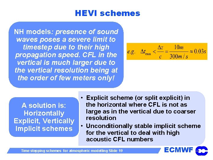
HEVI schemes NH models: presence of sound waves poses a severe limit to timestep due to their high propagation speed. CFL in the vertical is much larger due to the vertical resolution being at the order of few meters only! A solution is: Horizontally Explicit, Vertically Implicit schemes • Explicit scheme (or split explicit) in the horizontal where CFL is not as large as in the vertical due to coarser resolution • Unconditionally stable implicit scheme for the vertical to deal with high acoustic CFL numbers Time stepping schemes for atmospheric modelling Slide 19 ECMWF

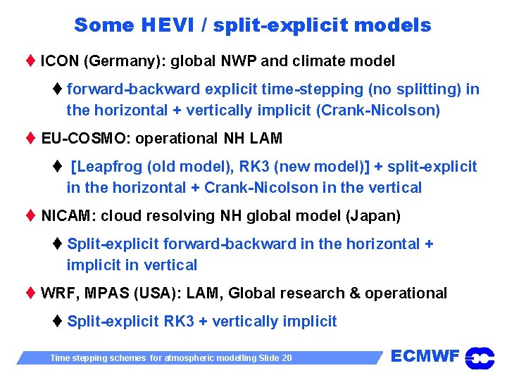
Some HEVI / split-explicit models t ICON (Germany): global NWP and climate model t forward-backward explicit time-stepping (no splitting) in the horizontal + vertically implicit (Crank-Nicolson) t EU-COSMO: operational NH LAM t [Leapfrog (old model), RK 3 (new model)] + split-explicit in the horizontal + Crank-Nicolson in the vertical t NICAM: cloud resolving NH global model (Japan) t Split-explicit forward-backward in the horizontal + implicit in vertical t WRF, MPAS (USA): LAM, Global research & operational t Split-explicit RK 3 + vertically implicit Time stepping schemes for atmospheric modelling Slide 20 ECMWF

Drawbacks of the split-explicit approach t In deep global NH models O(100 km) there is no much benefit from split-explicit approach in the horizontal t Stratospheric polar jet velocities not far from speed of sound advective CFL number almost as big as acoustic CFL number è Practically this means that all processes are fast and therefore horizontal splitting will not bring any efficiency benefit t Splitting needs damping for stabilization t Alternatives: t Implicit Explicit (IMEX) RK (unconditionally stable implicit scheme for fast processes and cheap explicit for slow) t IMEX has very general form: HEVI can be written as IMEX Time stepping schemes for atmospheric modelling Slide 21 ECMWF

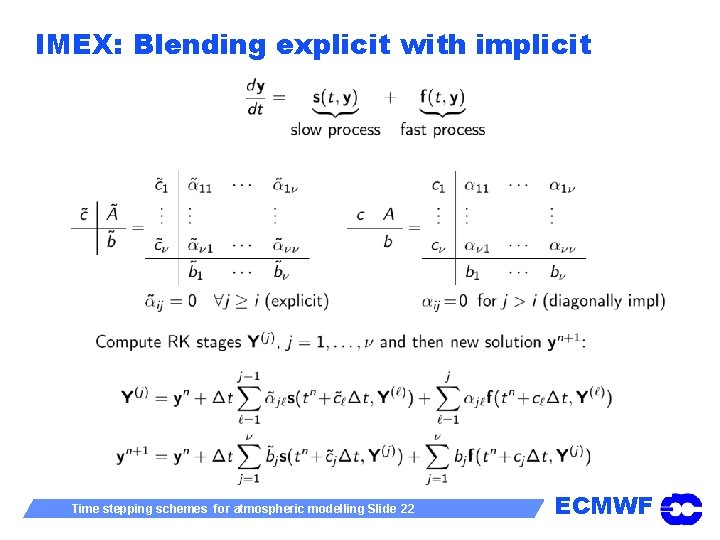
IMEX: Blending explicit with implicit Time stepping schemes for atmospheric modelling Slide 22 ECMWF

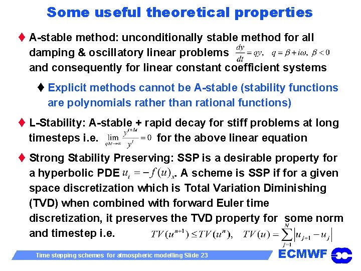
Some useful theoretical properties t A-stable method: unconditionally stable method for all damping & oscillatory linear problems and consequently for linear constant coefficient systems t Explicit methods cannot be A-stable (stability functions are polynomials rather than rational functions) t L-Stability: A-stable + rapid decay for stiff problems at long timesteps i. e. for the above linear equation t Strong Stability Preserving: SSP is a desirable property for a hyperbolic PDE. A scheme is SSP if for a given space discretization which is Total Variation Diminishing (TVD) when combined with forward Euler time discretization, it preserves the TVD property for some norm and timestep i. e. Time stepping schemes for atmospheric modelling Slide 23 ECMWF

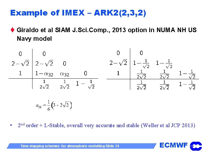
Example of IMEX – ARK 2(2, 3, 2) t Giraldo et al SIAM J. Sci. Comp. , 2013 option in NUMA NH US Navy model • 2 nd order + L-Stable, overall very accurate and stable (Weller et al JCP 2013) Time stepping schemes for atmospheric modelling Slide 24 ECMWF

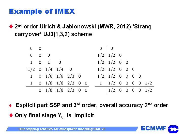
Example of IMEX t 2 nd order Ulrich & Jablonowski (MWR, 2012) ‘Strang carryover’ UJ 3(1, 3, 2) scheme t Explicit part SSP and 3 rd order, overall accuracy 2 nd order t Only final stage Y 6 is implicit Time stepping schemes for atmospheric modelling Slide 25 ECMWF

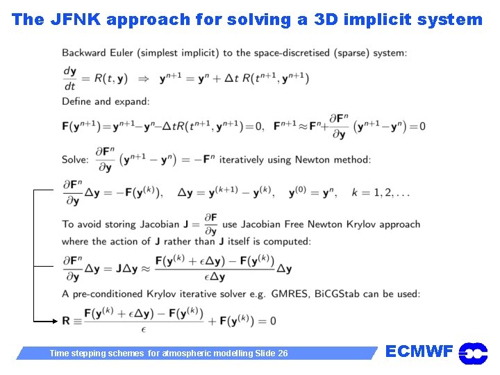
The JFNK approach for solving a 3 D implicit system Time stepping schemes for atmospheric modelling Slide 26 ECMWF

An emerging technique: exponential integrators Further reading: Luan et al, JCP Vol 376, Jan 2019, p 817 -837 Time stepping schemes for atmospheric modelling Slide 27 ECMWF

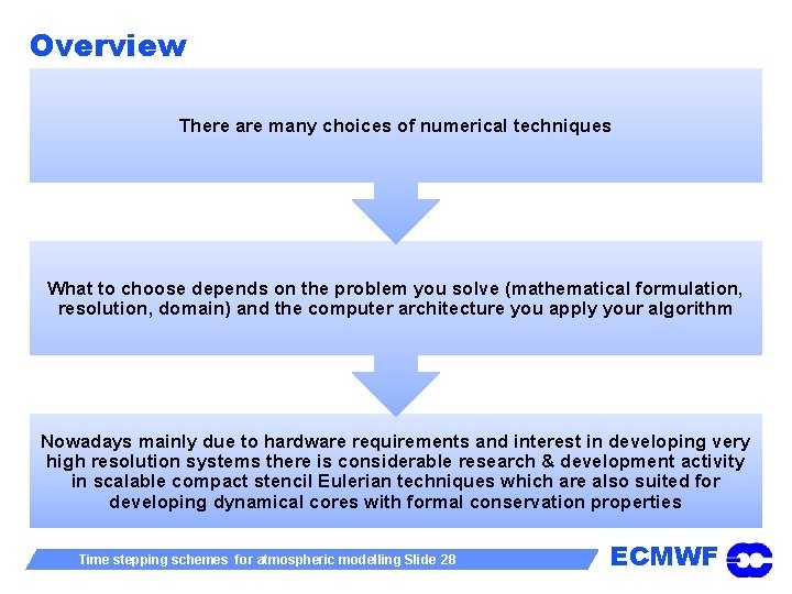
Overview There are many choices of numerical techniques What to choose depends on the problem you solve (mathematical formulation, resolution, domain) and the computer architecture you apply your algorithm Nowadays mainly due to hardware requirements and interest in developing very high resolution systems there is considerable research & development activity in scalable compact stencil Eulerian techniques which are also suited for developing dynamical cores with formal conservation properties Time stepping schemes for atmospheric modelling Slide 28 ECMWF

Some references t Dale Durran’s book: “Numerical methods for Wave Equations in Geophysical Fluid Dynamics” (1999) t Lauritzen et al book: Numerical Techniques for Global Atmospheric Models, Springer 2011 t Mengaldo et al, Archives of Comp. Meth. in Eng. (2018): Current and Emerging Time-Integration Strategies in Global NWP t Wicker & Skamarock (MWR 2001): “Time-Splitting Methods for Elastic Models Using Forward Time Schemes” Time stepping schemes for atmospheric modelling Slide 29 ECMWF

Thank you for your attention! Time stepping schemes for atmospheric modelling Slide 30 ECMWF