Time Series Econometrics Lecture 9 Cointegration and Error

Time Series Econometrics Lecture 9. Cointegration and Error Correction Models October 18 st , 2011 1

Announcements § Today is the last lecture! § Homework assignment # 3 deadline: November 1 st, 12 pm. Electronic version to be submitted to: calc_wiz@mail. ru § Exam: Winter exam session, January, 2012 § Consultation (time to be announced later): end of December 2

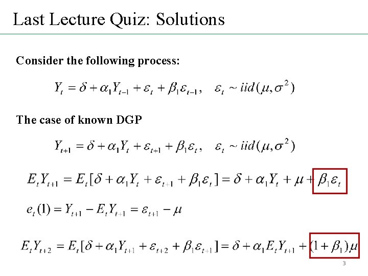
Last Lecture Quiz: Solutions Consider the following process: The case of known DGP 3

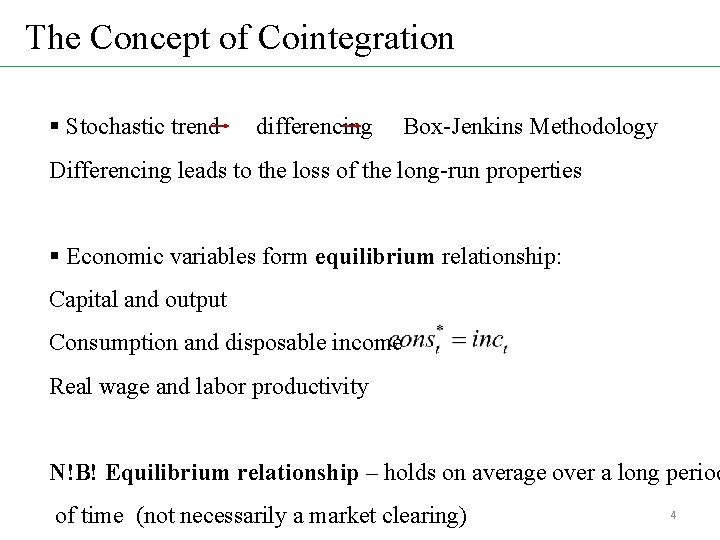
The Concept of Cointegration § Stochastic trend differencing Box-Jenkins Methodology Differencing leads to the loss of the long-run properties § Economic variables form equilibrium relationship: Capital and output Consumption and disposable income Real wage and labor productivity N!B! Equilibrium relationship – holds on average over a long period of time (not necessarily a market clearing) 4

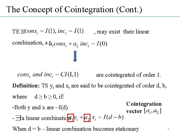
The Concept of Cointegration (Cont. ) TE If , may exist their linear combination, s. t. are cointegrated of order 1. Definition: TS yt and xt are said to be cointegrated of order d, b, where d ≥ b ≥ 0, if: -Both y and x are ~I(d) - Cointegration vector a linear combination When d = b – linear combination becomes stationary 5

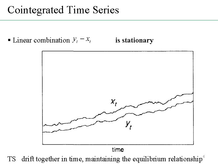
Cointegrated Time Series § Linear combination is stationary TS drift together in time, maintaining the equilibrium relationship 6

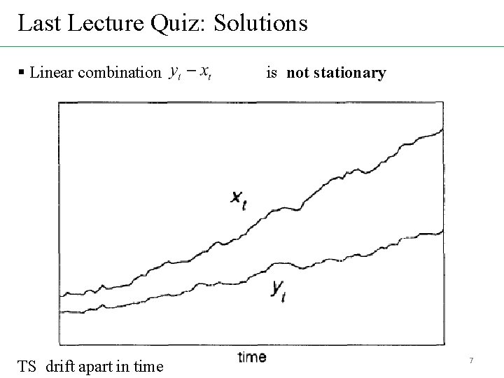
Last Lecture Quiz: Solutions § Linear combination TS drift apart in time is not stationary 7

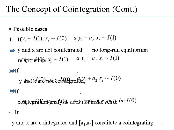
The Concept of Cointegration (Cont. ) § Possible cases 1. If , y and x are not cointegrated no long-run equilibrium relationship 2. If , y and x are not cointegrated; 3. If , cointegration analysis does not make sense 4. If , y and x are cointegrated and [a 1, a 2] constitute a cointegrating 8

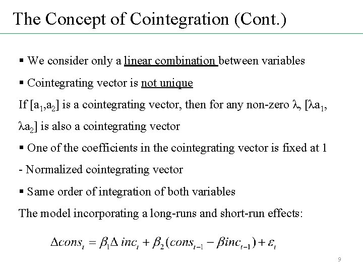
The Concept of Cointegration (Cont. ) § We consider only a linear combination between variables § Cointegrating vector is not unique If [a 1, a 2] is a cointegrating vector, then for any non-zero λ, [λa 1, λa 2] is also a cointegrating vector § One of the coefficients in the cointegrating vector is fixed at 1 - Normalized cointegrating vector § Same order of integration of both variables The model incorporating a long-runs and short-run effects: 9

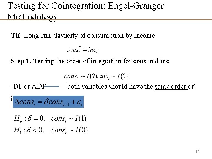
Testing for Cointegration: Engel-Granger Methodology TE Long-run elasticity of consumption by income Step 1. Testing the order of integration for cons and inc -DF or ADF both variables should have the same order of integration 10

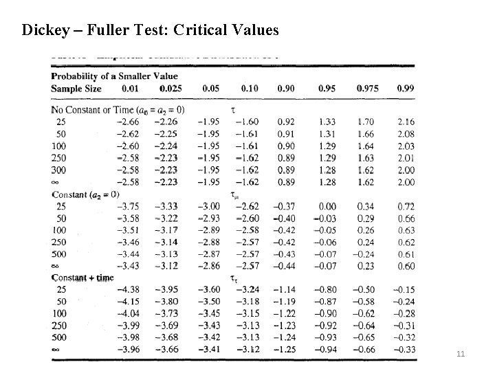
Dickey – Fuller Test: Critical Values 11

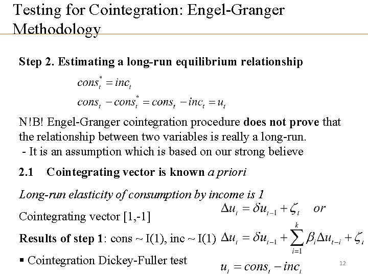
Testing for Cointegration: Engel-Granger Methodology Step 2. Estimating a long-run equilibrium relationship N!B! Engel-Granger cointegration procedure does not prove that the relationship between two variables is really a long-run. - It is an assumption which is based on our strong believe 2. 1 Cointegrating vector is known a priori Long-run elasticity of consumption by income is 1 Cointegrating vector [1, -1] Results of step 1: cons ~ I(1), inc ~ I(1) § Cointegration Dickey-Fuller test 12

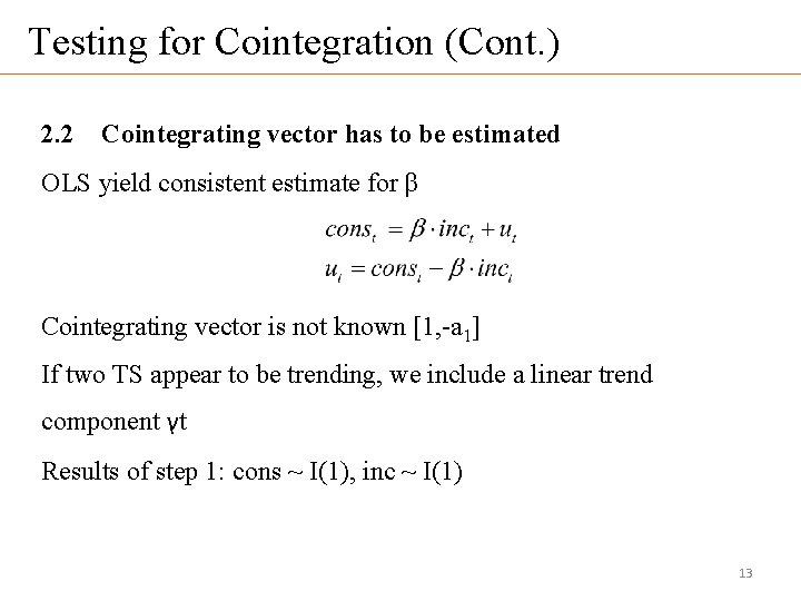
Testing for Cointegration (Cont. ) 2. 2 Cointegrating vector has to be estimated OLS yield consistent estimate for β Cointegrating vector is not known [1, -a 1] If two TS appear to be trending, we include a linear trend component γt Results of step 1: cons ~ I(1), inc ~ I(1) 13

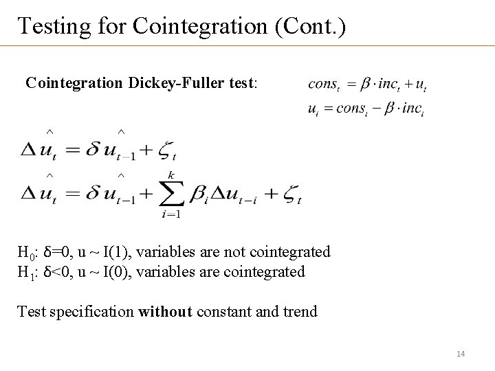
Testing for Cointegration (Cont. ) Cointegration Dickey-Fuller test: H 0: δ=0, u ~ I(1), variables are not cointegrated H 1: δ<0, u ~ I(0), variables are cointegrated Test specification without constant and trend 14

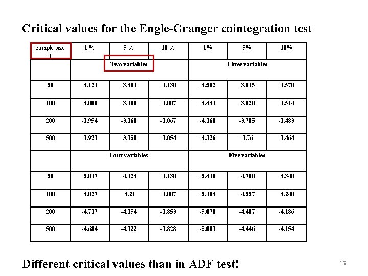
Critical values for the Engle-Granger cointegration test Sample size T 1% 5% 10 % 1% Two variables 5% 10% Three variables 50 -4. 123 -3. 461 -3. 130 -4. 592 -3. 915 -3. 578 100 -4. 008 -3. 398 -3. 087 -4. 441 -3. 828 -3. 514 200 -3. 954 -3. 368 -3. 067 -4. 368 -3. 785 -3. 483 500 -3. 921 -3. 350 -3. 054 -4. 326 -3. 76 -3. 464 Four variables Five variables 50 -5. 017 -4. 324 -3. 130 -5. 416 -4. 700 -4. 348 100 -4. 827 -4. 21 -3. 087 -5. 184 -4. 557 -4. 240 200 -4. 737 -4. 154 -3. 853 -5. 070 -4. 487 -4. 186 500 -4. 684 -4. 122 -3. 828 -5. 003 -4. 446 -4. 154 Different critical values than in ADF test! 15

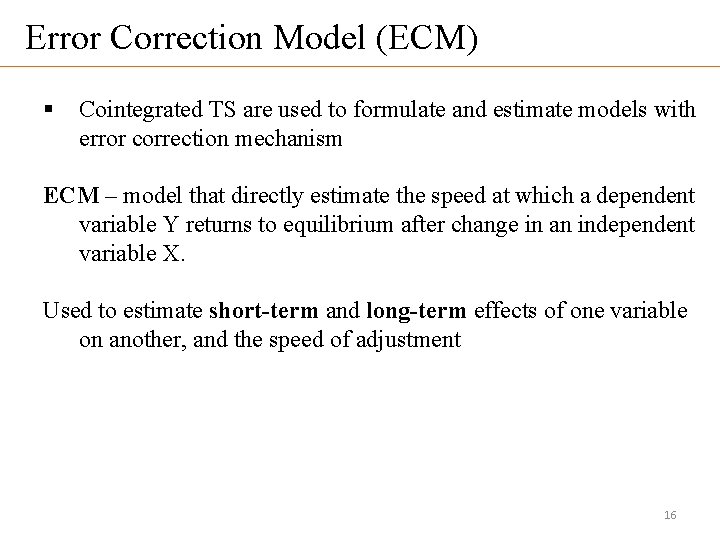
Error Correction Model (ECM) § Cointegrated TS are used to formulate and estimate models with error correction mechanism ECM – model that directly estimate the speed at which a dependent variable Y returns to equilibrium after change in an independent variable X. Used to estimate short-term and long-term effects of one variable on another, and the speed of adjustment 16

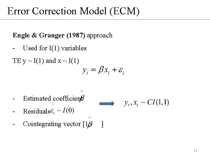
Error Correction Model (ECM) Engle & Granger (1987) approach - Used for I(1) variables TE y ~ I(1) and x ~ I(1) - Estimated coefficient - Residuals - Cointegrating vector [1, - ] 17

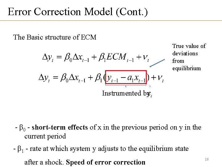
Error Correction Model (Cont. ) The Basic structure of ECM True value of deviations from equilibrium Instrumented by - β 0 - short-term effects of x in the previous period on y in the current period - β 1 - rate at which system y adjusts to the equilibrium state after a shock. Speed of error correction 18

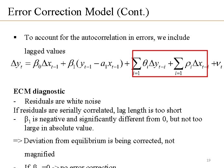
Error Correction Model (Cont. ) § To account for the autocorrelation in errors, we include lagged values ECM diagnostic - Residuals are white noise If residuals are serially correlated, lag length is too short - β 1 is negative and significantly different from 0, but not too large in absolute value. => Deviation from equilibrium is being corrected, not magnified 19

Assignment Reading assignment Charemza & Deadmam, pp. 122 -134 Homework assignment #3. Deadline: November 1 st, 12 pm. Submission in electronic form to the email: calc_wiz@mail. ru 20