Time Series Components Copyright c 2008 by The

Time Series Components Copyright (c) 2008 by The Mc. Graw-Hill Companies. This material is intended solely for educational use by licensed users of Learning. Stats. It may not be copied or resold for profit.

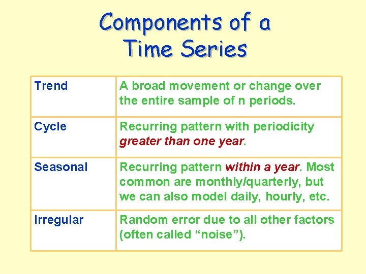
Components of a Time Series Trend A broad movement or change over the entire sample of n periods. Cycle Recurring pattern with periodicity greater than one year. Seasonal Recurring pattern within a year. Most common are monthly/quarterly, but we can also model daily, hourly, etc. Irregular Random error due to all other factors (often called “noise”).

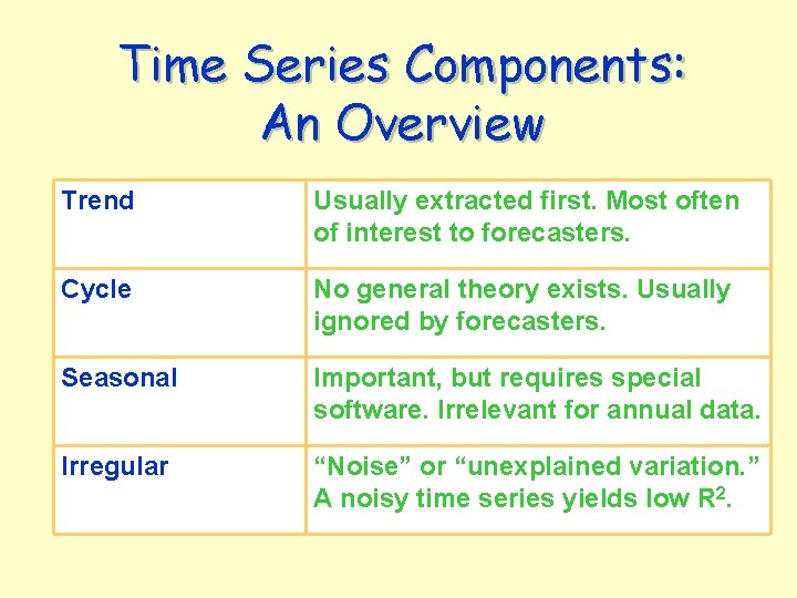
Time Series Components: An Overview Trend Usually extracted first. Most often of interest to forecasters. Cycle No general theory exists. Usually ignored by forecasters. Seasonal Important, but requires special software. Irrelevant for annual data. Irregular “Noise” or “unexplained variation. ” A noisy time series yields low R 2.

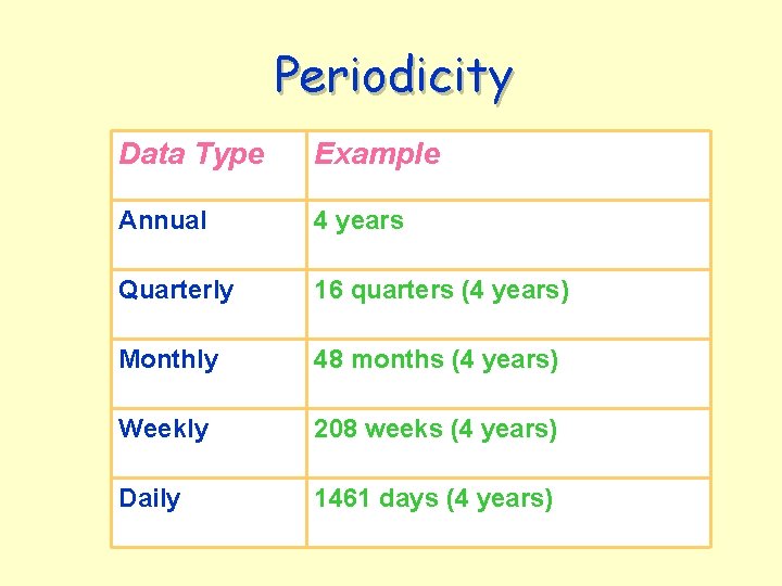
Periodicity Data Type Example Annual 4 years Quarterly 16 quarters (4 years) Monthly 48 months (4 years) Weekly 208 weeks (4 years) Daily 1461 days (4 years)

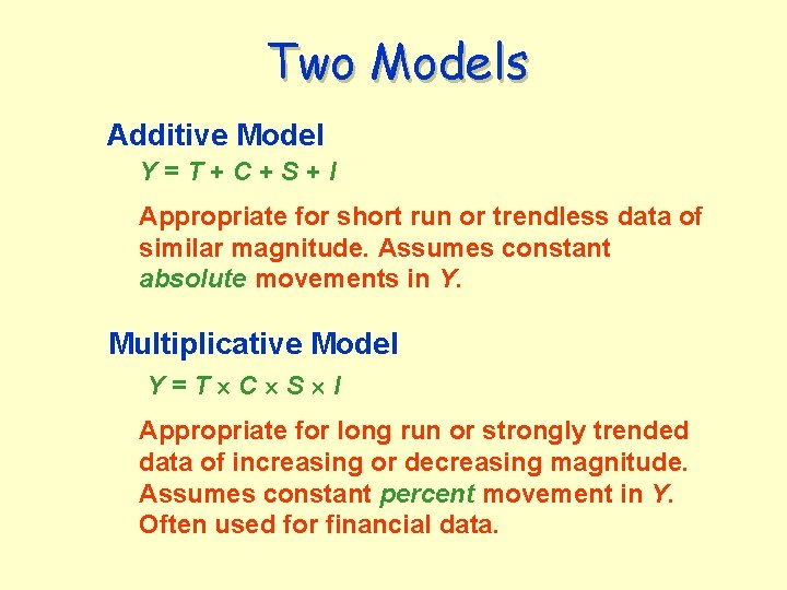
Two Models Additive Model Y=T+C+S+I Appropriate for short run or trendless data of similar magnitude. Assumes constant absolute movements in Y. Multiplicative Model Y=T C S I Appropriate for long run or strongly trended data of increasing or decreasing magnitude. Assumes constant percent movement in Y. Often used for financial data.

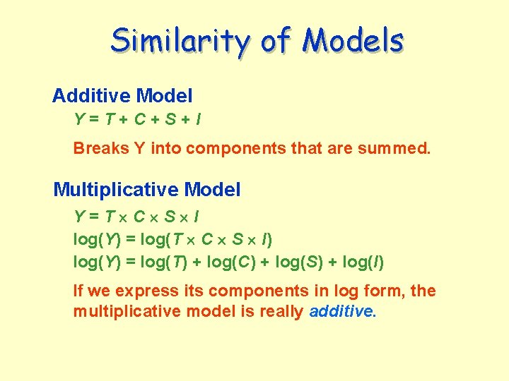
Similarity of Models Additive Model Y=T+C+S+I Breaks Y into components that are summed. Multiplicative Model Y=T C S I log(Y) = log(T C S I) log(Y) = log(T) + log(C) + log(S) + log(I) If we express its components in log form, the multiplicative model is really additive.

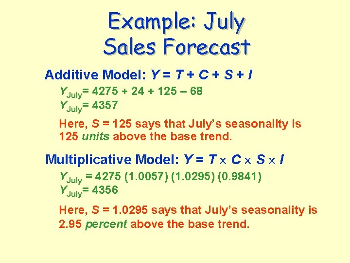
Example: July Sales Forecast Additive Model: Y = T + C + S + I YJuly= 4275 + 24 + 125 – 68 YJuly= 4357 Here, S = 125 says that July’s seasonality is 125 units above the base trend. Multiplicative Model: Y = T C S I YJuly = 4275 (1. 0057) (1. 0295) (0. 9841) YJuly= 4356 Here, S = 1. 0295 says that July’s seasonality is 2. 95 percent above the base trend.

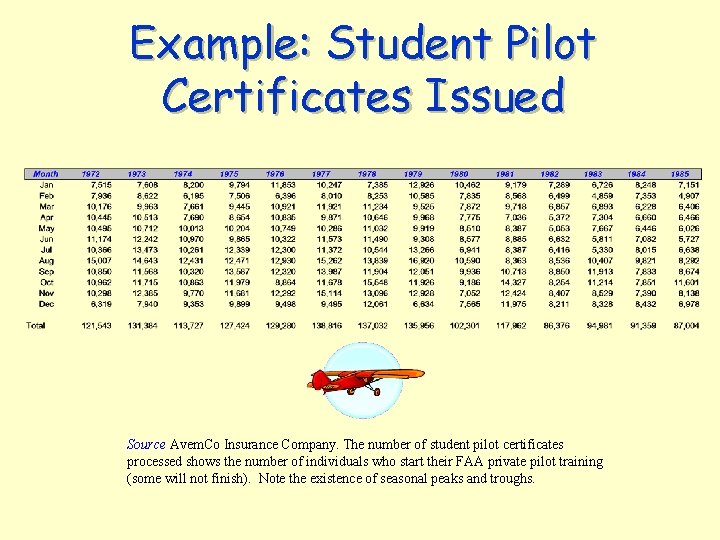
Example: Student Pilot Certificates Issued Source Avem. Co Insurance Company. The number of student pilot certificates processed shows the number of individuals who start their FAA private pilot training (some will not finish). Note the existence of seasonal peaks and troughs.

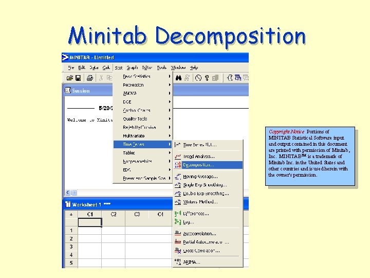
Minitab Decomposition Copyright Notice Portions of MINITAB Statistical Software input and output contained in this document are printed with permission of Minitab, Inc. MINITABTM is a trademark of Minitab Inc. in the United States and other countries and is used herein with the owner's permission.

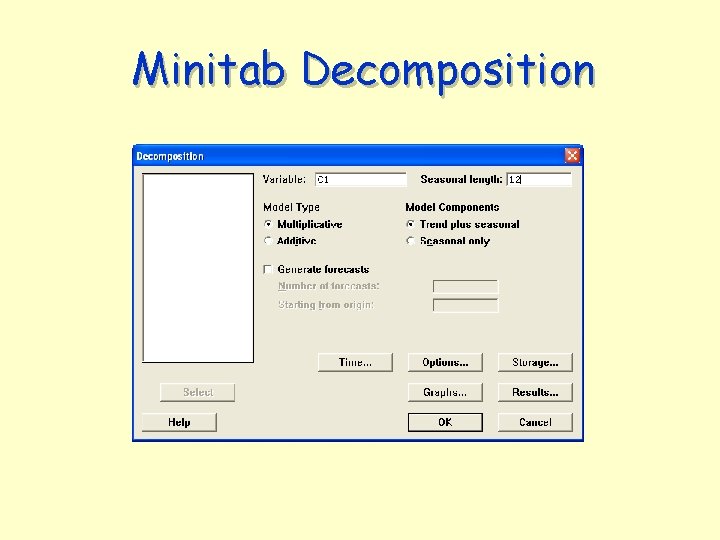
Minitab Decomposition

Minitab Decomposition Data are monthly U. S. student pilot certificates issued, 1972 -1985 (n = 168 months). Strong seasonality exists (seasonal spikes).

Minitab Decomposition Diagnostics for further analysis.

Decomposition: Advice v Excel doesn’t do it v But MINITAB does! v So do SPSS and SAS! Moral: Decomposition of monthly or quarterly time series data is not a task for a calculator or spreadsheet. Let specialized software handle it, and focus on interpreting the results.