Time Series and Forecasting Random Series STEREO XLS

Time Series and Forecasting Random Series

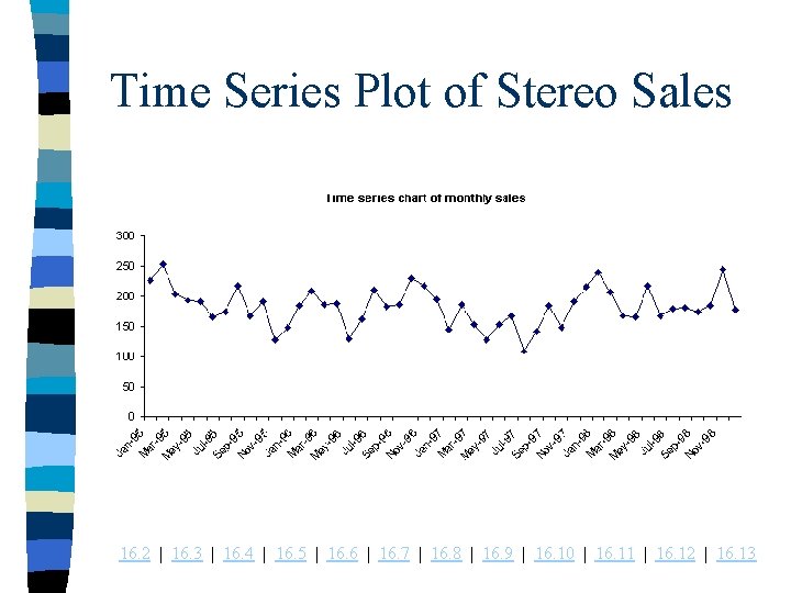
STEREO. XLS n Monthly sales for a chain of stereo retailers are listed in this file. n They cover the period form the beginning of 1995 to the end of 1998, during which there was no upward or downward trend in sales and no clear seasonal peaks or valleys. n This behavior is apparent in the time series chart of sales shown on the next slide. It is possible that this series is random. n Does a runs test support this conjecture? 16. 2 | 16. 3 | 16. 4 | 16. 5 | 16. 6 | 16. 7 | 16. 8 | 16. 9 | 16. 10 | 16. 11 | 16. 12 | 16. 13

Time Series Plot of Stereo Sales 16. 2 | 16. 3 | 16. 4 | 16. 5 | 16. 6 | 16. 7 | 16. 8 | 16. 9 | 16. 10 | 16. 11 | 16. 12 | 16. 13

Random Model n The simplest time series is the random model. n In a random model the observations vary around a constant mean, have a common variance, and are probabilistically independent of one another. n How can we tell whether a time series is random? n There are several checks that can be done individually or in tandem. n The first of these is to plot the series on a control chart. If the series is random it should be “in control”. 16. 2 | 16. 3 | 16. 4 | 16. 5 | 16. 6 | 16. 7 | 16. 8 | 16. 9 | 16. 10 | 16. 11 | 16. 12 | 16. 13

Runs Test n The runs test is the second check for a random series. n A run is a consecutive sequence of 0’s and 1’s. n The runs test checks whether this is about the right number of runs for a random series. 16. 2 | 16. 3 | 16. 4 | 16. 5 | 16. 6 | 16. 7 | 16. 8 | 16. 9 | 16. 10 | 16. 11 | 16. 12 | 16. 13

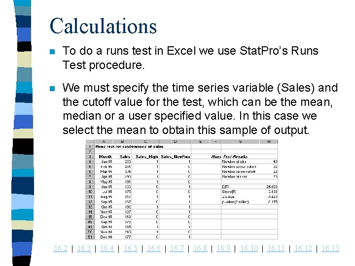
Calculations n To do a runs test in Excel we use Stat. Pro’s Runs Test procedure. n We must specify the time series variable (Sales) and the cutoff value for the test, which can be the mean, median or a user specified value. In this case we select the mean to obtain this sample of output. 16. 2 | 16. 3 | 16. 4 | 16. 5 | 16. 6 | 16. 7 | 16. 8 | 16. 9 | 16. 10 | 16. 11 | 16. 12 | 16. 13

Output n Note that Stat. Pro adds two new variables, Sales_High and Sales_New. Run, as well as the elements for the test. n The values in the Sales_High are 1 or 0 depending on whether the corresponding sales value are above or below the mean. n The values in the Sales_New. Run column are also 1 or 0, depending on whether a new run starts in that month. 16. 2 | 16. 3 | 16. 4 | 16. 5 | 16. 6 | 16. 7 | 16. 8 | 16. 9 | 16. 10 | 16. 11 | 16. 12 | 16. 13

Output -- continued n The rest of the output is fairly straightforward. n We find the number of observations above the mean, number of runs, mean for the observed number of runs, the standard deviation for the observed number of runs and the Z-value. We then can find the twosided p-value. n The output shows that there is some evidence of not enough runs. n The expected number of runs under randomness is 24. 8333 and there are only 20 runs for this series. 16. 2 | 16. 3 | 16. 4 | 16. 5 | 16. 6 | 16. 7 | 16. 8 | 16. 9 | 16. 10 | 16. 11 | 16. 12 | 16. 13

Conclusion n The conclusion is that sales do not tend to “zigzag” as much as a random series - highs tend to follow highs and lows tend to follow lows - but the evidence in favor of nonrandomness is not overwhelming. 16. 2 | 16. 3 | 16. 4 | 16. 5 | 16. 6 | 16. 7 | 16. 8 | 16. 9 | 16. 10 | 16. 11 | 16. 12 | 16. 13

Random Series

The Problem n The runs test on the stereo sales data suggests that the pattern of sales is not completely random. n Large values tend to follow large values, and small values tend to follow small values. n Do autocorrelations support this conclusion? 16. 2 | 16. 3 | 16. 4 | 16. 5 | 16. 6 | 16. 7 | 16. 8 | 16. 9 | 16. 10 | 16. 11 | 16. 12 | 16. 13

Autocorrelations n Recall that successive observations in a random series are probabilistically independent of one another. n Many time series violate this property and are instead autocorrelated. n The “auto” means that successive observations are correlated with one other. n To understand autocorrelations it is first necessary to understand what it means to lag a time series. 16. 2 | 16. 3 | 16. 4 | 16. 5 | 16. 6 | 16. 7 | 16. 8 | 16. 9 | 16. 10 | 16. 11 | 16. 12 | 16. 13

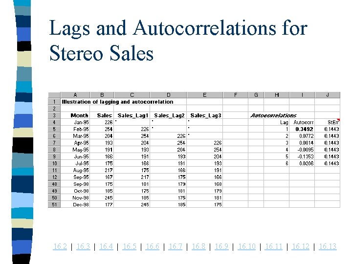
Autocorrelations n This concept is easy to understand in spreadsheets. n To lag by 1 month, we simply “push down” the series by one row. n Lags are simply previous observations, removed by a certain number of periods from the present time. 16. 2 | 16. 3 | 16. 4 | 16. 5 | 16. 6 | 16. 7 | 16. 8 | 16. 9 | 16. 10 | 16. 11 | 16. 12 | 16. 13

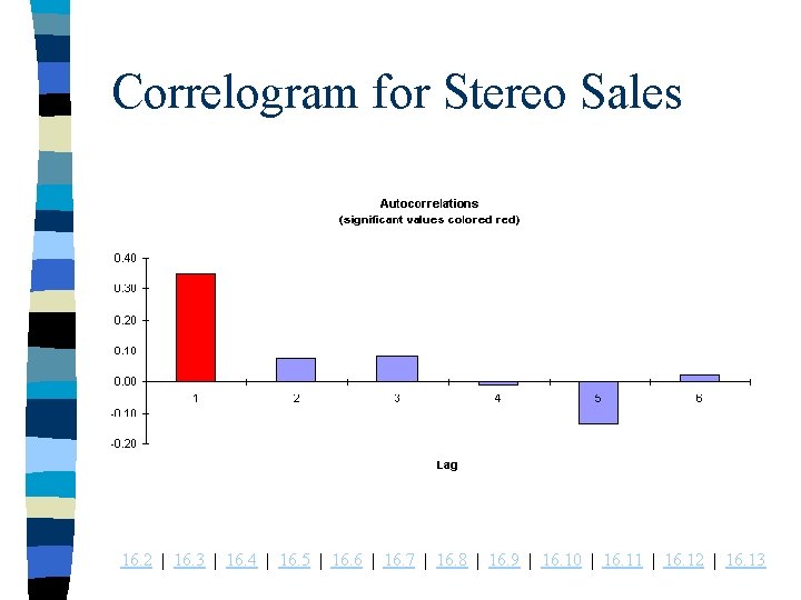
Solution n We use Stat. Pro’s Autocorrelation procedure. n This procedure requires us to specify a time series variable (Sales), the number of lags we want (we chose 6), and whether we want a chart of the autocorrelations. This chart is called a correlogram. n How large is a “large” autocorrelation? n If the series is truly random, then only an occasional autocorrelation should be larger than two standard errors in magnitude. 16. 2 | 16. 3 | 16. 4 | 16. 5 | 16. 6 | 16. 7 | 16. 8 | 16. 9 | 16. 10 | 16. 11 | 16. 12 | 16. 13

Solution -- continued n Therefore, any autocorrelation that is larger than two standard errors in magnitude is worth our attention. n The only “large” autocorrelation for the sales data is the first, or lag 1, the autocorrelation is 0. 3492. n The fact that it is positive indicates once again that there is some tendency for large sales values to follow large sales values and for small sales values to follow small sales values. n The autocorrelations are less than two standard errors in magnitude and can be considered “noise”. 16. 2 | 16. 3 | 16. 4 | 16. 5 | 16. 6 | 16. 7 | 16. 8 | 16. 9 | 16. 10 | 16. 11 | 16. 12 | 16. 13

Lags and Autocorrelations for Stereo Sales 16. 2 | 16. 3 | 16. 4 | 16. 5 | 16. 6 | 16. 7 | 16. 8 | 16. 9 | 16. 10 | 16. 11 | 16. 12 | 16. 13

Correlogram for Stereo Sales 16. 2 | 16. 3 | 16. 4 | 16. 5 | 16. 6 | 16. 7 | 16. 8 | 16. 9 | 16. 10 | 16. 11 | 16. 12 | 16. 13

Random Series

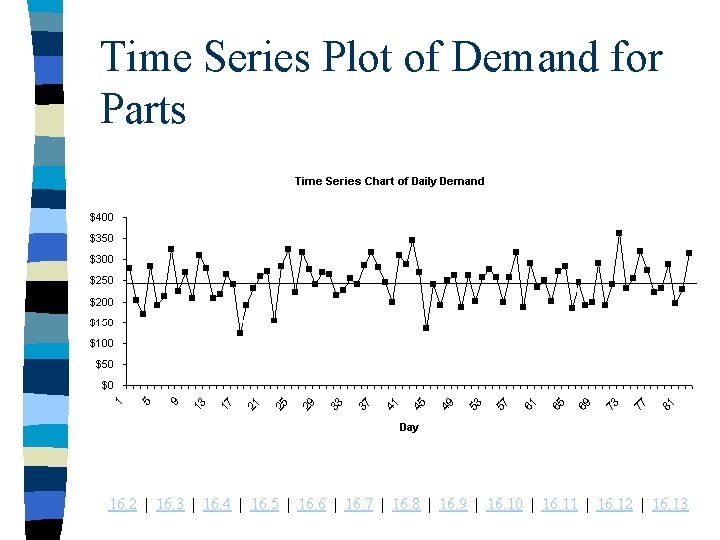
DEMAND. XLS n The dollar demand for a certain class of parts at a local retail store has been recorded for 82 consecutive days. n This file contains the recorded data. n The store manager wants to forecast future demands. n In particular, he wants to know whethere is any significant time pattern to the historical demands or whether the series is essentially random. 16. 2 | 16. 3 | 16. 4 | 16. 5 | 16. 6 | 16. 7 | 16. 8 | 16. 9 | 16. 10 | 16. 11 | 16. 12 | 16. 13

Time Series Plot of Demand for Parts 16. 2 | 16. 3 | 16. 4 | 16. 5 | 16. 6 | 16. 7 | 16. 8 | 16. 9 | 16. 10 | 16. 11 | 16. 12 | 16. 13

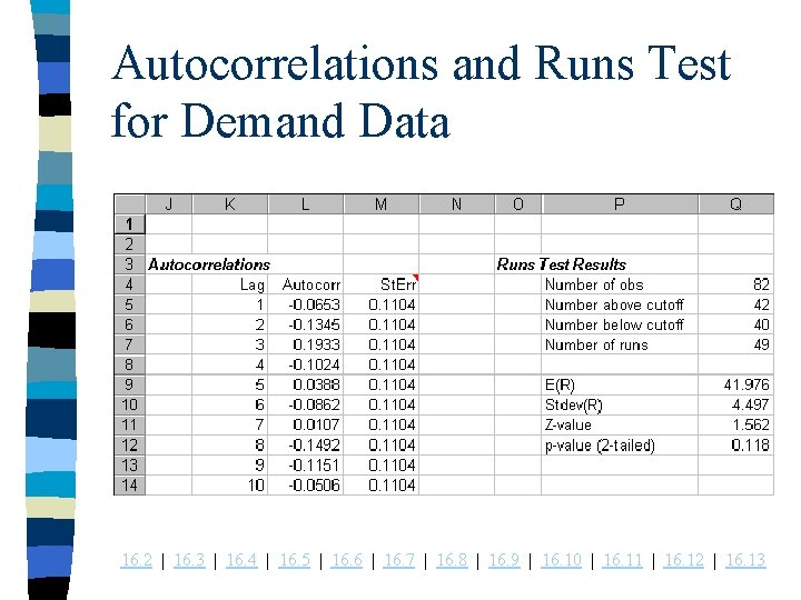
Solution n A visual inspection of the time series graph shows that demands vary randomly around the sample mean of $247. 54 (shown as the horizontal centerline). n The variance appears to be constant through time, and there are no obvious time series patterns. n To check formally whether this apparent randomness holds, we perform the runs test and calculate the first 10 autocorrelations. The numerical output and associated correlogram are shown on the next slides. 16. 2 | 16. 3 | 16. 4 | 16. 5 | 16. 6 | 16. 7 | 16. 8 | 16. 9 | 16. 10 | 16. 11 | 16. 12 | 16. 13

Autocorrelations and Runs Test for Demand Data 16. 2 | 16. 3 | 16. 4 | 16. 5 | 16. 6 | 16. 7 | 16. 8 | 16. 9 | 16. 10 | 16. 11 | 16. 12 | 16. 13

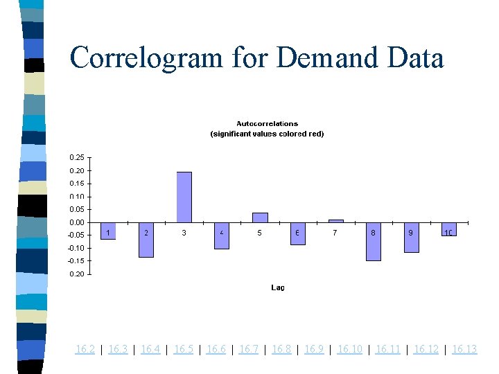
Correlogram for Demand Data 16. 2 | 16. 3 | 16. 4 | 16. 5 | 16. 6 | 16. 7 | 16. 8 | 16. 9 | 16. 10 | 16. 11 | 16. 12 | 16. 13

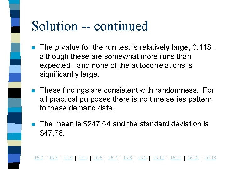
Solution -- continued n The p-value for the run test is relatively large, 0. 118 although these are somewhat more runs than expected - and none of the autocorrelations is significantly large. n These findings are consistent with randomness. For all practical purposes there is no time series pattern to these demand data. n The mean is $247. 54 and the standard deviation is $47. 78. 16. 2 | 16. 3 | 16. 4 | 16. 5 | 16. 6 | 16. 7 | 16. 8 | 16. 9 | 16. 10 | 16. 11 | 16. 12 | 16. 13

Solution -- continued n The manager might as well forecast that demand for any day in the future will be $247. 54. If he does so about 95% of his forecast should be within two standard deviations (about $95) of the actual demands. 16. 2 | 16. 3 | 16. 4 | 16. 5 | 16. 6 | 16. 7 | 16. 8 | 16. 9 | 16. 10 | 16. 11 | 16. 12 | 16. 13

The Random Walk Model

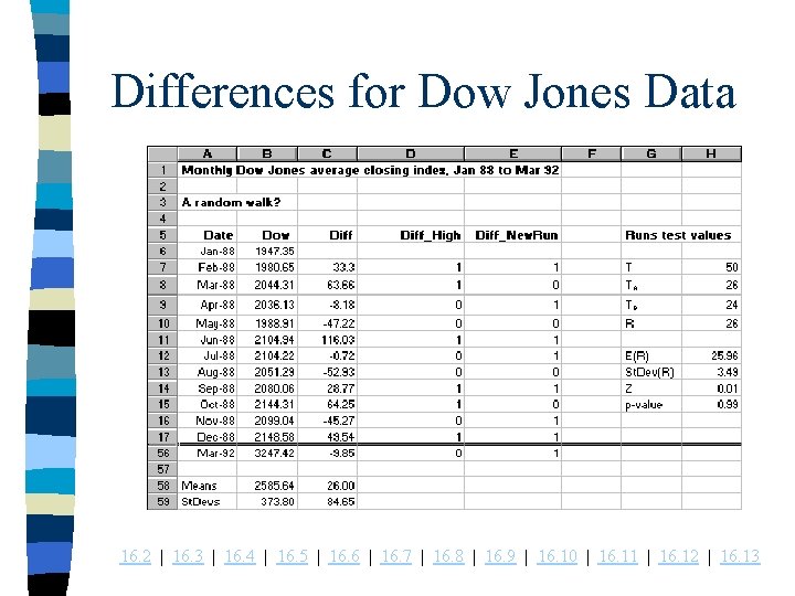
DOW. XLS n Given the monthly Dow Jones data in this file, check that it satisfies the assumptions of a random walk, and use the random walk model to forecast the value for April 1992. 16. 2 | 16. 3 | 16. 4 | 16. 5 | 16. 6 | 16. 7 | 16. 8 | 16. 9 | 16. 10 | 16. 11 | 16. 12 | 16. 13

Random Walk Model n Random series are sometimes building blocks for other time series models. n The random walk model is an example of this. n In the random walk model the series itself is not random. However, its differences - that is the changes from one period to the next - are random. n This type of behavior is typical of stock price data. 16. 2 | 16. 3 | 16. 4 | 16. 5 | 16. 6 | 16. 7 | 16. 8 | 16. 9 | 16. 10 | 16. 11 | 16. 12 | 16. 13

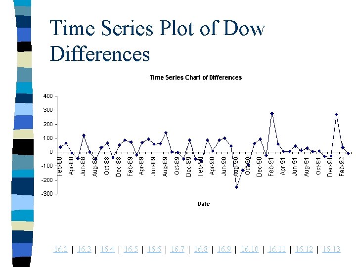
Solution n The Dow Jones series itself is not random, due to upward trend, so we form the differences in Column C with the formula =B 7 -B 6 which is copied down column C. The difference can be seen on the next slide. n A graph of the differences (see graph following data) show the series to be a much more random series, varying around the mean difference 26. 00. n The runs test appears in column H and shows that there is absolutely no evidence of nonrandom differences; the observed number of runs is almost identical to the expected number. 16. 2 | 16. 3 | 16. 4 | 16. 5 | 16. 6 | 16. 7 | 16. 8 | 16. 9 | 16. 10 | 16. 11 | 16. 12 | 16. 13

Differences for Dow Jones Data 16. 2 | 16. 3 | 16. 4 | 16. 5 | 16. 6 | 16. 7 | 16. 8 | 16. 9 | 16. 10 | 16. 11 | 16. 12 | 16. 13

Time Series Plot of Dow Differences 16. 2 | 16. 3 | 16. 4 | 16. 5 | 16. 6 | 16. 7 | 16. 8 | 16. 9 | 16. 10 | 16. 11 | 16. 12 | 16. 13

Solution -- continued n Similarly, the autocorrelations are all small except for a random “blip” at lag 11. n Because the values are 11 months apart we would tend to ignore this autocorrelation. n Assuming the random walk model is adequate, the forecast of April 1992 made in March 1992 is the observed March value, 3247. 42, plus the mean difference, 26. 00 or 3273. 42. n A measure of the forecast accuracy is the standard deviation of 84. 65. We can be 95% certain that our forecast will be within the standard deviations. 16. 2 | 16. 3 | 16. 4 | 16. 5 | 16. 6 | 16. 7 | 16. 8 | 16. 9 | 16. 10 | 16. 11 | 16. 12 | 16. 13

Additional Forecasting n If we wanted to forecast further into the future, say 3 months, based on the data through March 1992, we would add the most recent value, 3247. 42, to three times the mean difference, 26. 00. n That is, we just project the trend that far into the future. n We caution about forecasting too far into the future for such a volatile series as the Dow. 16. 2 | 16. 3 | 16. 4 | 16. 5 | 16. 6 | 16. 7 | 16. 8 | 16. 9 | 16. 10 | 16. 11 | 16. 12 | 16. 13

Autoregressive Models

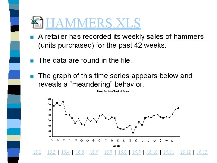
HAMMERS. XLS n A retailer has recorded its weekly sales of hammers (units purchased) for the past 42 weeks. n The data are found in the file. n The graph of this time series appears below and reveals a “meandering” behavior. 16. 2 | 16. 3 | 16. 4 | 16. 5 | 16. 6 | 16. 7 | 16. 8 | 16. 9 | 16. 10 | 16. 11 | 16. 12 | 16. 13

The Plot and Data n The values begin high and stay high awhile, then get lower and stay lower awhile, then get higher again. n This behavior could be caused by any number of things. n How useful is autoregression for modeling these data and how would it be used forecasting? 16. 2 | 16. 3 | 16. 4 | 16. 5 | 16. 6 | 16. 7 | 16. 8 | 16. 9 | 16. 10 | 16. 11 | 16. 12 | 16. 13

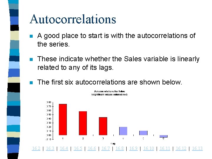
Autocorrelations n A good place to start is with the autocorrelations of the series. n These indicate whether the Sales variable is linearly related to any of its lags. n The first six autocorrelations are shown below. 16. 2 | 16. 3 | 16. 4 | 16. 5 | 16. 6 | 16. 7 | 16. 8 | 16. 9 | 16. 10 | 16. 11 | 16. 12 | 16. 13

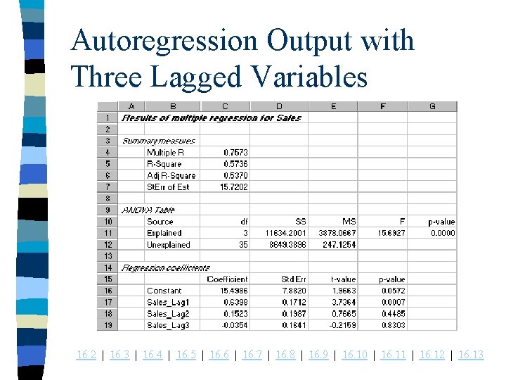
Autocorrelations -- continued n The first three of them are significantly positive, and then they decrease. n Based on this information, we create three lags of Sales and run a regression of Sales versus these three lags. n Here is the output from this regression 16. 2 | 16. 3 | 16. 4 | 16. 5 | 16. 6 | 16. 7 | 16. 8 | 16. 9 | 16. 10 | 16. 11 | 16. 12 | 16. 13

Autoregression Output with Three Lagged Variables 16. 2 | 16. 3 | 16. 4 | 16. 5 | 16. 6 | 16. 7 | 16. 8 | 16. 9 | 16. 10 | 16. 11 | 16. 12 | 16. 13

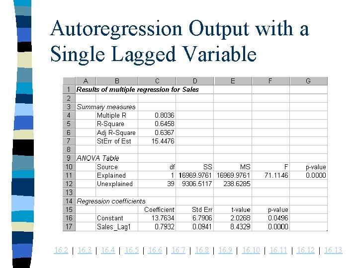
Autocorrelations -- continued n We see that R 2 is fairly high, about 57%, and that se is about 15. 7. n However, the p-values for lags 2 and 3 are both quite large. n It appears that once the first lag is included in the regression equation, the other two are not really needed. n Therefore we reran the regression with only the first lag include. 16. 2 | 16. 3 | 16. 4 | 16. 5 | 16. 6 | 16. 7 | 16. 8 | 16. 9 | 16. 10 | 16. 11 | 16. 12 | 16. 13

Autoregression Output with a Single Lagged Variable 16. 2 | 16. 3 | 16. 4 | 16. 5 | 16. 6 | 16. 7 | 16. 8 | 16. 9 | 16. 10 | 16. 11 | 16. 12 | 16. 13

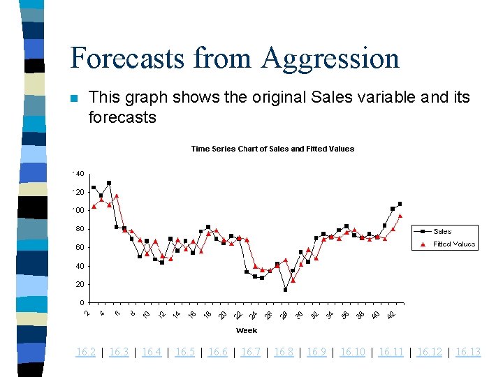
Forecasts from Aggression n This graph shows the original Sales variable and its forecasts 16. 2 | 16. 3 | 16. 4 | 16. 5 | 16. 6 | 16. 7 | 16. 8 | 16. 9 | 16. 10 | 16. 11 | 16. 12 | 16. 13

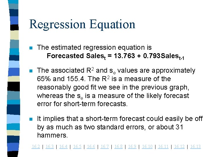
Regression Equation n The estimated regression equation is Forecasted Salest = 13. 763 + 0. 793 Salest-1 n The associated R 2 and se values are approximately 65% and 155. 4. The R 2 is a measure of the reasonably good fit we see in the previous graph, whereas the se is a measure of the likely forecast error for short-term forecasts. n It implies that a short-term forecast could easily be off by as much as two standard errors, or about 31 hammers. 16. 2 | 16. 3 | 16. 4 | 16. 5 | 16. 6 | 16. 7 | 16. 8 | 16. 9 | 16. 10 | 16. 11 | 16. 12 | 16. 13

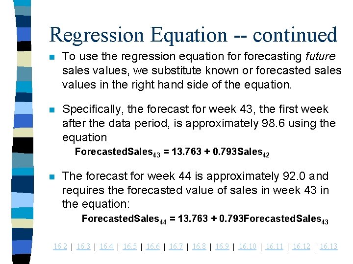
Regression Equation -- continued n To use the regression equation forecasting future sales values, we substitute known or forecasted sales values in the right hand side of the equation. n Specifically, the forecast for week 43, the first week after the data period, is approximately 98. 6 using the equation Forecasted. Sales 43 = 13. 763 + 0. 793 Sales 42 n The forecast for week 44 is approximately 92. 0 and requires the forecasted value of sales in week 43 in the equation: Forecasted. Sales 44 = 13. 763 + 0. 793 Forecasted. Sales 43 16. 2 | 16. 3 | 16. 4 | 16. 5 | 16. 6 | 16. 7 | 16. 8 | 16. 9 | 16. 10 | 16. 11 | 16. 12 | 16. 13

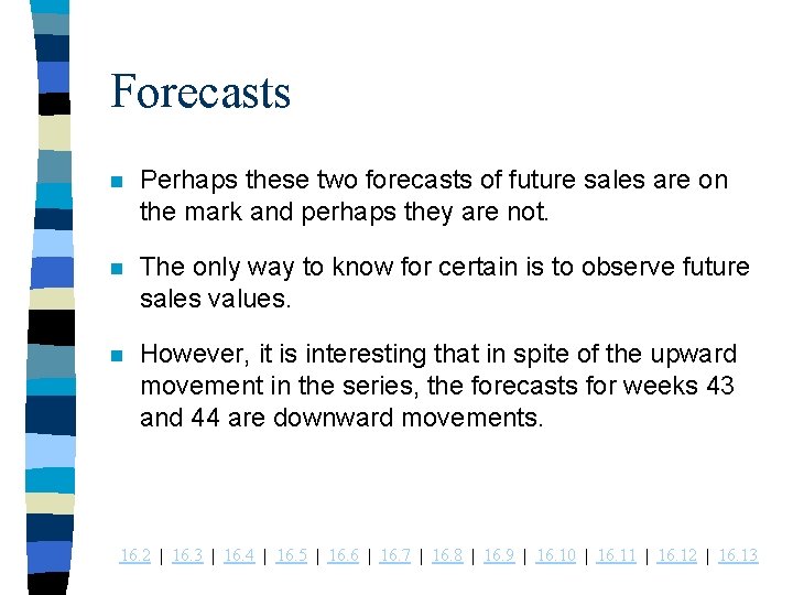
Forecasts n Perhaps these two forecasts of future sales are on the mark and perhaps they are not. n The only way to know for certain is to observe future sales values. n However, it is interesting that in spite of the upward movement in the series, the forecasts for weeks 43 and 44 are downward movements. 16. 2 | 16. 3 | 16. 4 | 16. 5 | 16. 6 | 16. 7 | 16. 8 | 16. 9 | 16. 10 | 16. 11 | 16. 12 | 16. 13

Regression Equation Properties n The downward trend is caused by a combination of the two properties of the regression equation. n First, the coefficient of Salest-1, 0. 793, is positive. Therefore the equation forecasts that large sales will be followed by large sales (that is, positive autocorrelation). n Second, however, this coefficient is less than 1, and this provides a dampening effect. n The equation forecasts that a large will follow a large, but not that large. 16. 2 | 16. 3 | 16. 4 | 16. 5 | 16. 6 | 16. 7 | 16. 8 | 16. 9 | 16. 10 | 16. 11 | 16. 12 | 16. 13

Regression-Based Trend Models

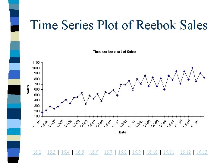
REEBOK. XLS n This file includes quarterly sales data for Reebok from first quarter 1986 through second quarter 1996. n The following screen shows the time series plot of these data. n Sales increase from $174. 52 million in the first quarter to $817. 57 million in the final quarter. n How well does a linear trend fit these data? n Are the residuals from this fit random? 16. 2 | 16. 3 | 16. 4 | 16. 5 | 16. 6 | 16. 7 | 16. 8 | 16. 9 | 16. 10 | 16. 11 | 16. 12 | 16. 13

Time Series Plot of Reebok Sales 16. 2 | 16. 3 | 16. 4 | 16. 5 | 16. 6 | 16. 7 | 16. 8 | 16. 9 | 16. 10 | 16. 11 | 16. 12 | 16. 13

Linear Trend n A linear trend means that the time series variable changes by a constant amount each time period. n The relevant equation is Yt = a + bt + Et where a is the intercept, b is the slope and Et is an error term. n If b is positive the trend is upward, if b is negative then the trend is downward. n The graph of the time series is a good place to start. It indicates whether a linear trend model is likely to provide a good fit. 16. 2 | 16. 3 | 16. 4 | 16. 5 | 16. 6 | 16. 7 | 16. 8 | 16. 9 | 16. 10 | 16. 11 | 16. 12 | 16. 13

Solution n The plot indicates an obvious upward trend with little or no curvature. n Therefore, a linear trend is certainly plausible. n We use regression to estimate the linear fit, where Sales is the response variable and Time is the single explanatory variable. n The Time variable is coded 1 -42 and is used as the explanatory variable in the regression. 16. 2 | 16. 3 | 16. 4 | 16. 5 | 16. 6 | 16. 7 | 16. 8 | 16. 9 | 16. 10 | 16. 11 | 16. 12 | 16. 13

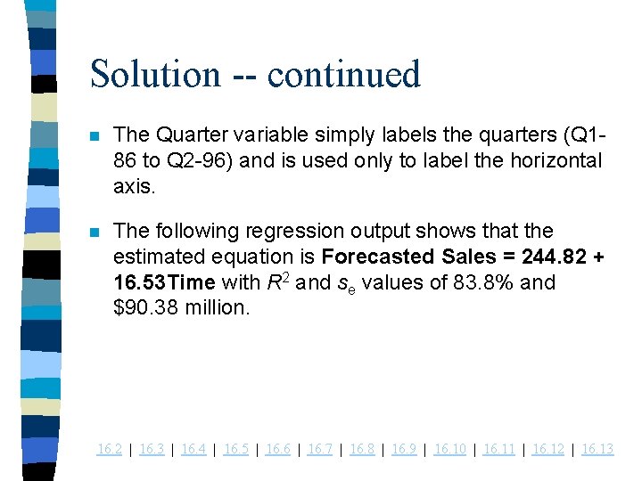
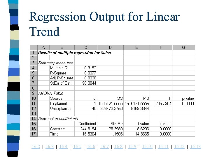
Solution -- continued n The Quarter variable simply labels the quarters (Q 186 to Q 2 -96) and is used only to label the horizontal axis. n The following regression output shows that the estimated equation is Forecasted Sales = 244. 82 + 16. 53 Time with R 2 and se values of 83. 8% and $90. 38 million. 16. 2 | 16. 3 | 16. 4 | 16. 5 | 16. 6 | 16. 7 | 16. 8 | 16. 9 | 16. 10 | 16. 11 | 16. 12 | 16. 13

Regression Output for Linear Trend 16. 2 | 16. 3 | 16. 4 | 16. 5 | 16. 6 | 16. 7 | 16. 8 | 16. 9 | 16. 10 | 16. 11 | 16. 12 | 16. 13

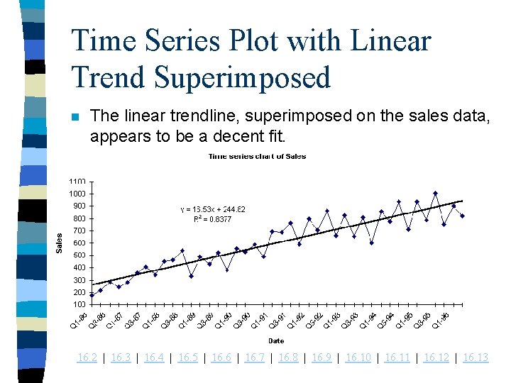
Time Series Plot with Linear Trend Superimposed n The linear trendline, superimposed on the sales data, appears to be a decent fit. 16. 2 | 16. 3 | 16. 4 | 16. 5 | 16. 6 | 16. 7 | 16. 8 | 16. 9 | 16. 10 | 16. 11 | 16. 12 | 16. 13

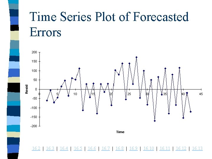
Solution -- continued n The trendline implies that sales are increasing by about $16. 53 million per quarter during this period. n The fit is far from perfect, however. – First, the se value $90. 38 million is an indication of the typical forecast error. This is substantial, approximately equal to 11% of the final quarter’s sales – Furthermore, there is some regularity to the forecast errors shown in the following plot. 16. 2 | 16. 3 | 16. 4 | 16. 5 | 16. 6 | 16. 7 | 16. 8 | 16. 9 | 16. 10 | 16. 11 | 16. 12 | 16. 13

Time Series Plot of Forecasted Errors 16. 2 | 16. 3 | 16. 4 | 16. 5 | 16. 6 | 16. 7 | 16. 8 | 16. 9 | 16. 10 | 16. 11 | 16. 12 | 16. 13

Plot Interpretation n They zigzag more than a random series. n There is probably some seasonal pattern in the sales data, which we might be able to pick up with a more sophisticated forecasting method. n However, the basic linear trend is sufficient as a first approximation to the behavior of sales. 16. 2 | 16. 3 | 16. 4 | 16. 5 | 16. 6 | 16. 7 | 16. 8 | 16. 9 | 16. 10 | 16. 11 | 16. 12 | 16. 13

Regression-Based Trend Models

INTEL. XLS n This file contains quarterly sales data for the chip manufacturing firm Intel from the beginning of 1986 through the second quarter of 1996. n Each sales value is expressed in millions of dollars. n Check that an exponential trend fits these sales data fairly well. n Then estimate the relationship and interpret it. 16. 2 | 16. 3 | 16. 4 | 16. 5 | 16. 6 | 16. 7 | 16. 8 | 16. 9 | 16. 10 | 16. 11 | 16. 12 | 16. 13

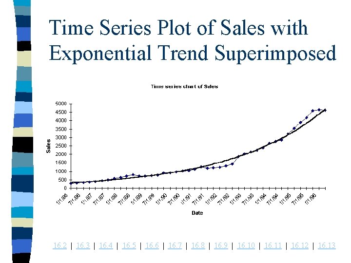
Time Series Plot of Sales with Exponential Trend Superimposed 16. 2 | 16. 3 | 16. 4 | 16. 5 | 16. 6 | 16. 7 | 16. 8 | 16. 9 | 16. 10 | 16. 11 | 16. 12 | 16. 13

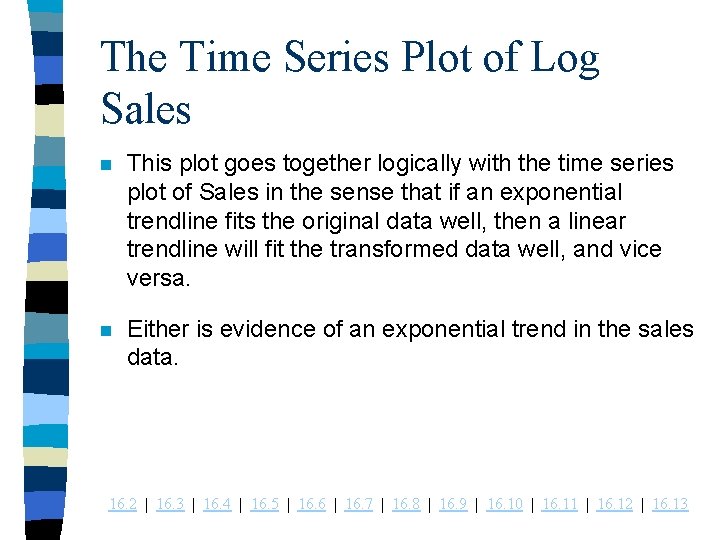
The Time Series Plot of Sales n The time series plot shows that sales are clearly increasing at an increasing rate, which a linear trend would not capture. n The smooth curve of the plot is an exponential trendline, which appears to be an adequate fit. n Alternatively, we can try to “straighten out” the data by taking the log of sales with Excel’s LN function. n The following is a plot of the log data. 16. 2 | 16. 3 | 16. 4 | 16. 5 | 16. 6 | 16. 7 | 16. 8 | 16. 9 | 16. 10 | 16. 11 | 16. 12 | 16. 13

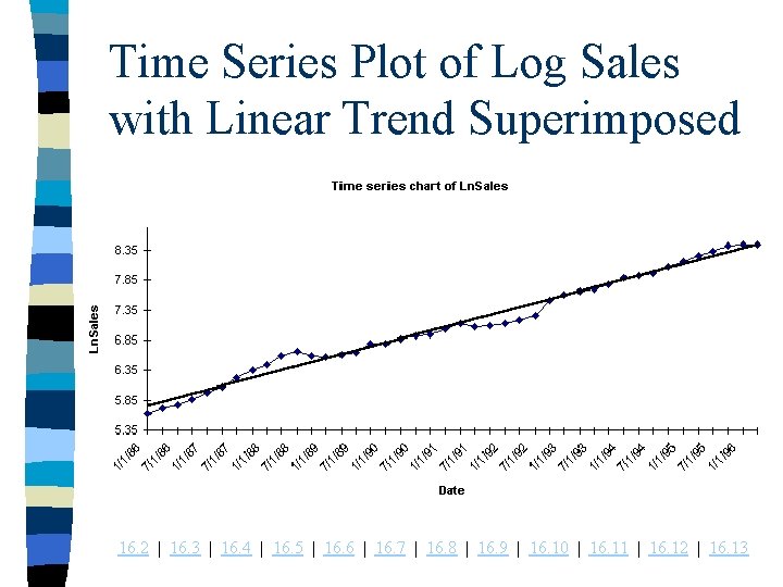
Time Series Plot of Log Sales with Linear Trend Superimposed 16. 2 | 16. 3 | 16. 4 | 16. 5 | 16. 6 | 16. 7 | 16. 8 | 16. 9 | 16. 10 | 16. 11 | 16. 12 | 16. 13

The Time Series Plot of Log Sales n This plot goes together logically with the time series plot of Sales in the sense that if an exponential trendline fits the original data well, then a linear trendline will fit the transformed data well, and vice versa. n Either is evidence of an exponential trend in the sales data. 16. 2 | 16. 3 | 16. 4 | 16. 5 | 16. 6 | 16. 7 | 16. 8 | 16. 9 | 16. 10 | 16. 11 | 16. 12 | 16. 13

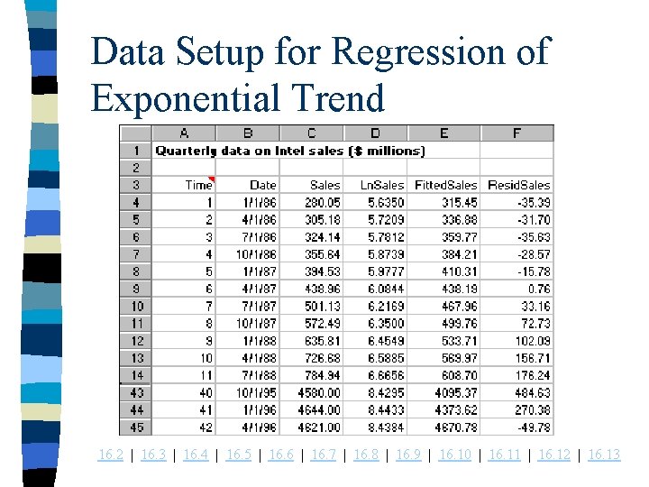
Estimating the Exponential Trend n To estimate the exponential trend, we run a regression of the log of sales, Ln. Sales, versus Time. n A portion of the resulting data and output appears below. 16. 2 | 16. 3 | 16. 4 | 16. 5 | 16. 6 | 16. 7 | 16. 8 | 16. 9 | 16. 10 | 16. 11 | 16. 12 | 16. 13

Data Setup for Regression of Exponential Trend 16. 2 | 16. 3 | 16. 4 | 16. 5 | 16. 6 | 16. 7 | 16. 8 | 16. 9 | 16. 10 | 16. 11 | 16. 12 | 16. 13

Regression Output for Exponential Trend 16. 2 | 16. 3 | 16. 4 | 16. 5 | 16. 6 | 16. 7 | 16. 8 | 16. 9 | 16. 10 | 16. 11 | 16. 12 | 16. 13

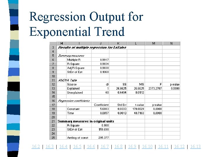
Regression Output n The regression output shows that the estimated log of sales is given by Forecasted Ln. Sales = 5. 6883 + 0. 0657 Time n Looking at the coefficient of Time, we can say that Intel’s sales are increasing by approximately 6. 6% per quarter during this period. n This translates to an annual percentage increase of about 29%. Perhaps the slight tailing off that we see at the right indicates that Intel can’t keep up this fantastic rate forever. 16. 2 | 16. 3 | 16. 4 | 16. 5 | 16. 6 | 16. 7 | 16. 8 | 16. 9 | 16. 10 | 16. 11 | 16. 12 | 16. 13

Regression Output -- continued n It is important to view the R 2 and se values with caution. Each is based in log units not original units. n To produce similar measures in original units, we need to forecast sales in Column E. This is a two step process. – First, we forecast the log sales. – Then we take the antilog with Excel’s EXP function. The specific formula is =EXP($J$18+$J$19*A 4). 16. 2 | 16. 3 | 16. 4 | 16. 5 | 16. 6 | 16. 7 | 16. 8 | 16. 9 | 16. 10 | 16. 11 | 16. 12 | 16. 13

Regression Output -- continued n As usual, R 2 is the square of the correlation between actual and fitted sales values, so the formula in cell J 22 is =CORREL(Sales, Fitted. Sales)ˆ2. n Then se is the square root of the sum of squared residuals divided by n-2. We can calculate this in cell J 23 by using Excel’s SUMSQ(sum of squares) function: =SQRT(SUMSQ(Resid. SAles)/40). n The R 2 value of 0. 988 indicates that there is a very high correlation between the actual and fitted sales values. In other words, the exponential fit is a very good one. 16. 2 | 16. 3 | 16. 4 | 16. 5 | 16. 6 | 16. 7 | 16. 8 | 16. 9 | 16. 10 | 16. 11 | 16. 12 | 16. 13

Regression Output -- continued n However, the se value if 159. 698 (in millions of dollars) indicates the forecasts based on this exponential fit could still be fairly far off. 16. 2 | 16. 3 | 16. 4 | 16. 5 | 16. 6 | 16. 7 | 16. 8 | 16. 9 | 16. 10 | 16. 11 | 16. 12 | 16. 13

Moving Averages

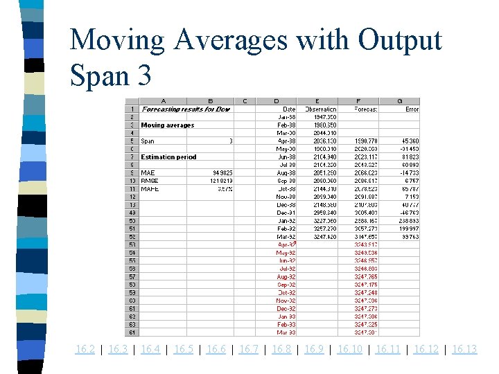
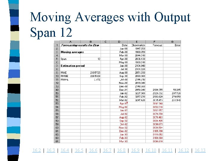
DOW. XLS n We again look at the Dow Jones monthly data from January 1988 through March 1992 contained in this file. n How well do moving averages track this series when the span is 23 months; when the span is 12 months? n What about future forecasts, that is, beyond March 1992? 16. 2 | 16. 3 | 16. 4 | 16. 5 | 16. 6 | 16. 7 | 16. 8 | 16. 9 | 16. 10 | 16. 11 | 16. 12 | 16. 13

Moving Averages n Perhaps the simplest and one of the most frequently used extrapolation methods is the method of moving averages. n To implement the moving averages method, we first choose a span, the number of terms in each moving average. n The role of span is very important. If the span is large - say 12 months - then many observations go into each average, and extreme values have relatively little effect on the forecasts. 16. 2 | 16. 3 | 16. 4 | 16. 5 | 16. 6 | 16. 7 | 16. 8 | 16. 9 | 16. 10 | 16. 11 | 16. 12 | 16. 13

Moving Averages -- continued n The resulting series forecasts will be much smoother than the original series. n For this reason the moving average method is called a smoothing method. 16. 2 | 16. 3 | 16. 4 | 16. 5 | 16. 6 | 16. 7 | 16. 8 | 16. 9 | 16. 10 | 16. 11 | 16. 12 | 16. 13

Moving Averages Method in Excel n Although the moving averages method is quite easy to implement with Excel, it can be tedious. n Therefore we can use the Forecasting procedure of Stat. Pro. This procedure lets us forecast with many methods. n We’ll go through the entire procedure step by step. 16. 2 | 16. 3 | 16. 4 | 16. 5 | 16. 6 | 16. 7 | 16. 8 | 16. 9 | 16. 10 | 16. 11 | 16. 12 | 16. 13

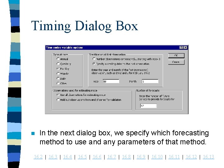
Forecasting Procedure n To use the Stat. Pro Forecasting procedure, the cursor needs to be in a data set with time series data. n We use the Stat. Pro/Forecasting menu item and eventually choose Dow as the variable to analyze. n We then see several dialog boxes, the first of which is where we specify the timing. 16. 2 | 16. 3 | 16. 4 | 16. 5 | 16. 6 | 16. 7 | 16. 8 | 16. 9 | 16. 10 | 16. 11 | 16. 12 | 16. 13

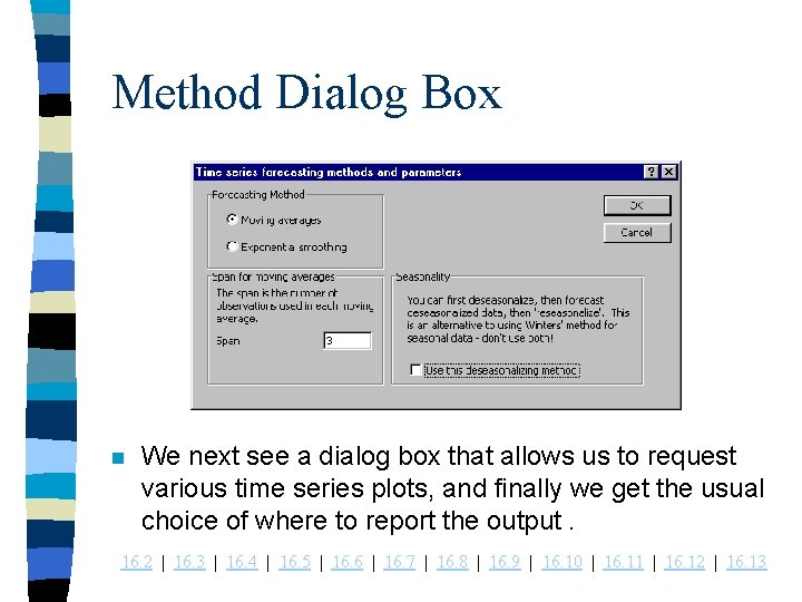
Timing Dialog Box n In the next dialog box, we specify which forecasting method to use and any parameters of that method. 16. 2 | 16. 3 | 16. 4 | 16. 5 | 16. 6 | 16. 7 | 16. 8 | 16. 9 | 16. 10 | 16. 11 | 16. 12 | 16. 13

Method Dialog Box n We next see a dialog box that allows us to request various time series plots, and finally we get the usual choice of where to report the output. 16. 2 | 16. 3 | 16. 4 | 16. 5 | 16. 6 | 16. 7 | 16. 8 | 16. 9 | 16. 10 | 16. 11 | 16. 12 | 16. 13

The Output n The output consists of several parts. n First, the forecasts and forecast errors are shown for the historical period of data. n Actually, with moving averages we lose some forecasts at the beginning of the period. n If we ask for future forecasts, they are shown in red at the bottom of the data series. n There are no forecast errors and to the left we see the summary measures. 16. 2 | 16. 3 | 16. 4 | 16. 5 | 16. 6 | 16. 7 | 16. 8 | 16. 9 | 16. 10 | 16. 11 | 16. 12 | 16. 13

Moving Averages with Output Span 3 16. 2 | 16. 3 | 16. 4 | 16. 5 | 16. 6 | 16. 7 | 16. 8 | 16. 9 | 16. 10 | 16. 11 | 16. 12 | 16. 13

Moving Averages with Output Span 12 16. 2 | 16. 3 | 16. 4 | 16. 5 | 16. 6 | 16. 7 | 16. 8 | 16. 9 | 16. 10 | 16. 11 | 16. 12 | 16. 13

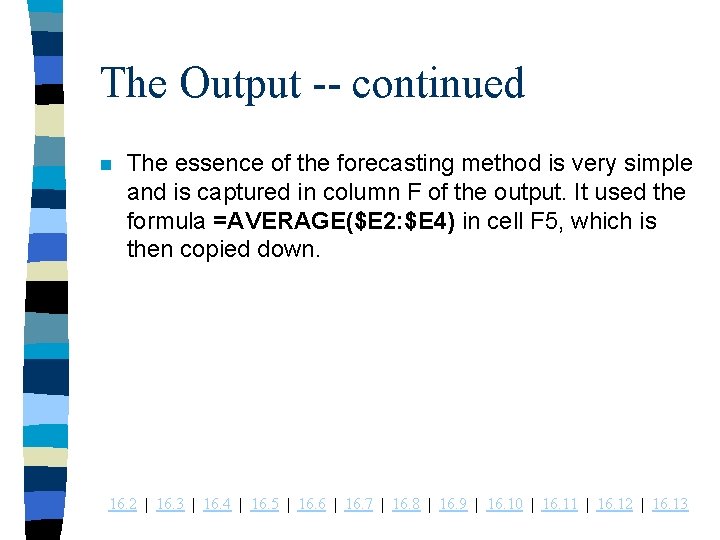
The Output -- continued n The essence of the forecasting method is very simple and is captured in column F of the output. It used the formula =AVERAGE($E 2: $E 4) in cell F 5, which is then copied down. 16. 2 | 16. 3 | 16. 4 | 16. 5 | 16. 6 | 16. 7 | 16. 8 | 16. 9 | 16. 10 | 16. 11 | 16. 12 | 16. 13

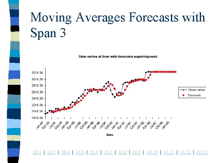
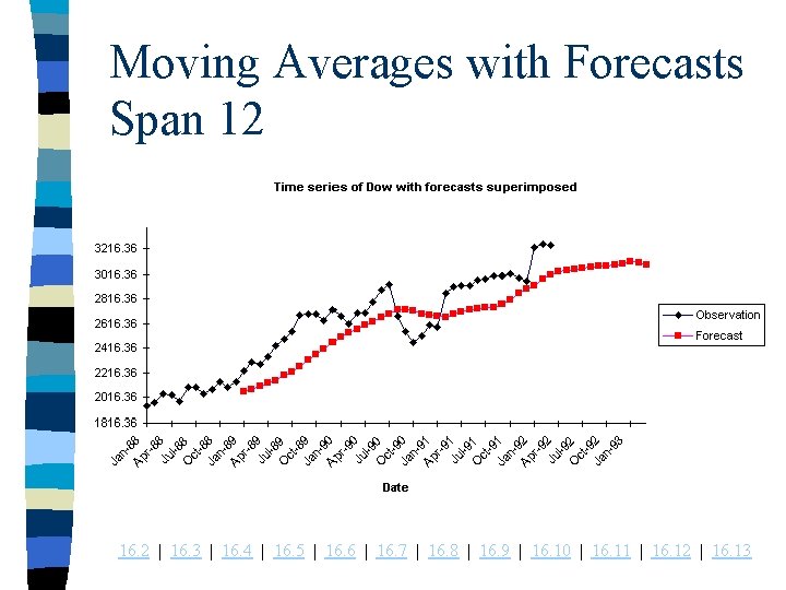
The Plots n The plots show the behavior of the forecasts. n The forecasts with span 3 appear to track the data better, whereas the forecasts with span 12 is considerably smoother - it reacts less to ups and downs of the series. 16. 2 | 16. 3 | 16. 4 | 16. 5 | 16. 6 | 16. 7 | 16. 8 | 16. 9 | 16. 10 | 16. 11 | 16. 12 | 16. 13

Moving Averages Forecasts with Span 3 16. 2 | 16. 3 | 16. 4 | 16. 5 | 16. 6 | 16. 7 | 16. 8 | 16. 9 | 16. 10 | 16. 11 | 16. 12 | 16. 13

Moving Averages with Forecasts Span 12 16. 2 | 16. 3 | 16. 4 | 16. 5 | 16. 6 | 16. 7 | 16. 8 | 16. 9 | 16. 10 | 16. 11 | 16. 12 | 16. 13

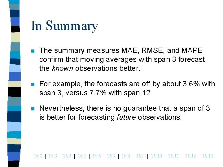
In Summary n The summary measures MAE, RMSE, and MAPE confirm that moving averages with span 3 forecast the known observations better. n For example, the forecasts are off by about 3. 6% with span 3, versus 7. 7% with span 12. n Nevertheless, there is no guarantee that a span of 3 is better forecasting future observations. 16. 2 | 16. 3 | 16. 4 | 16. 5 | 16. 6 | 16. 7 | 16. 8 | 16. 9 | 16. 10 | 16. 11 | 16. 12 | 16. 13

Exponential Smoothing

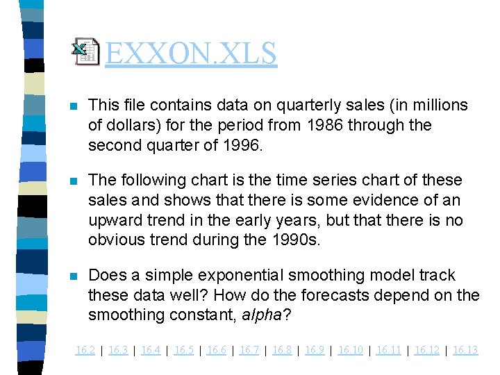
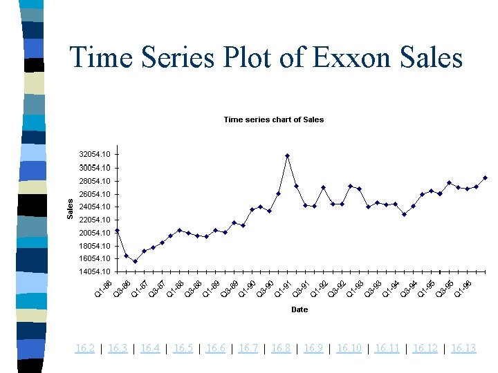
EXXON. XLS n This file contains data on quarterly sales (in millions of dollars) for the period from 1986 through the second quarter of 1996. n The following chart is the time series chart of these sales and shows that there is some evidence of an upward trend in the early years, but that there is no obvious trend during the 1990 s. n Does a simple exponential smoothing model track these data well? How do the forecasts depend on the smoothing constant, alpha? 16. 2 | 16. 3 | 16. 4 | 16. 5 | 16. 6 | 16. 7 | 16. 8 | 16. 9 | 16. 10 | 16. 11 | 16. 12 | 16. 13

Time Series Plot of Exxon Sales 16. 2 | 16. 3 | 16. 4 | 16. 5 | 16. 6 | 16. 7 | 16. 8 | 16. 9 | 16. 10 | 16. 11 | 16. 12 | 16. 13

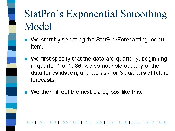
Stat. Pro’s Exponential Smoothing Model n We start by selecting the Stat. Pro/Forecasting menu item. n We first specify that the data are quarterly, beginning in quarter 1 of 1986, we do not hold out any of the data for validation, and we ask for 8 quarters of future forecasts. n We then fill out the next dialog box like this: 16. 2 | 16. 3 | 16. 4 | 16. 5 | 16. 6 | 16. 7 | 16. 8 | 16. 9 | 16. 10 | 16. 11 | 16. 12 | 16. 13

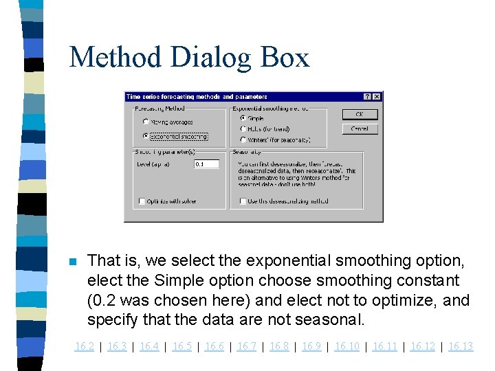
Method Dialog Box n That is, we select the exponential smoothing option, elect the Simple option choose smoothing constant (0. 2 was chosen here) and elect not to optimize, and specify that the data are not seasonal. 16. 2 | 16. 3 | 16. 4 | 16. 5 | 16. 6 | 16. 7 | 16. 8 | 16. 9 | 16. 10 | 16. 11 | 16. 12 | 16. 13

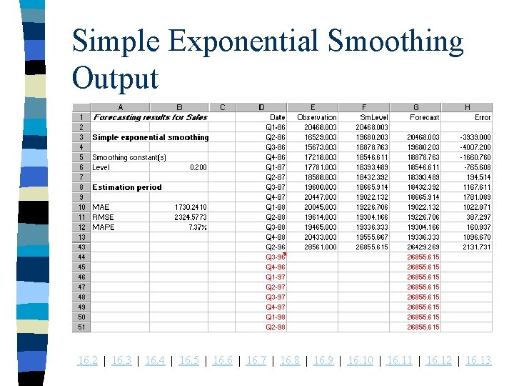
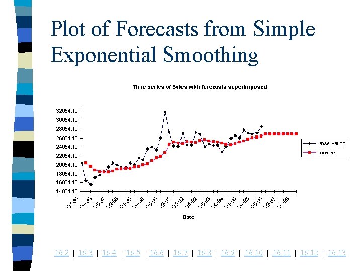
Stat. Pro’s Exponential Smoothing Model -- continued n On the next dialog sheet we ask for time series charts of the series with the forecasts superimposed and the series of forecast errors. n The results appear in the following three figures. n The heart of the method takes place in the columns F, G, and H of the first figure. The following formulas are used in row 6 of these columns. =Alpha*E 6+(1 -Alpha)*F 5 =E 6 -G 6 16. 2 | 16. 3 | 16. 4 | 16. 5 | 16. 6 | 16. 7 | 16. 8 | 16. 9 | 16. 10 | 16. 11 | 16. 12 | 16. 13

Stat. Pro’s Exponential Smoothing Model -- continued n The one exception to this scheme is in row 2. – Every exponential smoothing method requires initial values, in this case the initial smoothed level in cell F 2. – There is no way to calculate this value because the previous value is unknown. n Note that 8 future forecasts are all equal to the last calculated smoothed level in cell F 43. – The fact that these remain constant is a consequence of the assumption behind simple exponential smoothing, namely, that the series is not really going anywhere. Therefore, the last smoothed level is the best indication of future values of the series we have. 16. 2 | 16. 3 | 16. 4 | 16. 5 | 16. 6 | 16. 7 | 16. 8 | 16. 9 | 16. 10 | 16. 11 | 16. 12 | 16. 13

Simple Exponential Smoothing Output 16. 2 | 16. 3 | 16. 4 | 16. 5 | 16. 6 | 16. 7 | 16. 8 | 16. 9 | 16. 10 | 16. 11 | 16. 12 | 16. 13

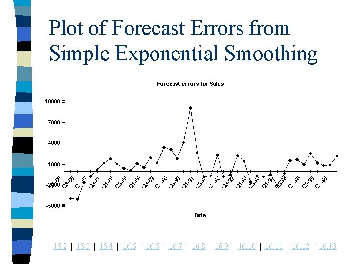
Forecast Series & Error Charts n The next figure shows the forecast series superimposed on the original series. n We see the obvious smoothing effect of a relatively small alpha level. n The forecasts don’t track the series well; but if the zig zags are just random noise, then we don’t want the forecasts to track these random ups and downs too closely. n A plot of the forecast errors shows some quite large errors, yet the errors do appear to be fairly random. 16. 2 | 16. 3 | 16. 4 | 16. 5 | 16. 6 | 16. 7 | 16. 8 | 16. 9 | 16. 10 | 16. 11 | 16. 12 | 16. 13

Plot of Forecasts from Simple Exponential Smoothing 16. 2 | 16. 3 | 16. 4 | 16. 5 | 16. 6 | 16. 7 | 16. 8 | 16. 9 | 16. 10 | 16. 11 | 16. 12 | 16. 13

Plot of Forecast Errors from Simple Exponential Smoothing 16. 2 | 16. 3 | 16. 4 | 16. 5 | 16. 6 | 16. 7 | 16. 8 | 16. 9 | 16. 10 | 16. 11 | 16. 12 | 16. 13

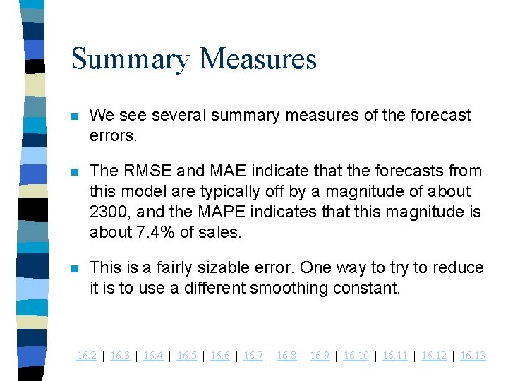
Summary Measures n We several summary measures of the forecast errors. n The RMSE and MAE indicate that the forecasts from this model are typically off by a magnitude of about 2300, and the MAPE indicates that this magnitude is about 7. 4% of sales. n This is a fairly sizable error. One way to try to reduce it is to use a different smoothing constant. 16. 2 | 16. 3 | 16. 4 | 16. 5 | 16. 6 | 16. 7 | 16. 8 | 16. 9 | 16. 10 | 16. 11 | 16. 12 | 16. 13

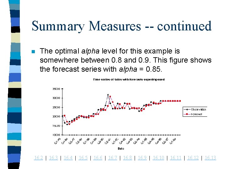
Summary Measures -- continued n The optimal alpha level for this example is somewhere between 0. 8 and 0. 9. This figure shows the forecast series with alpha = 0. 85. 16. 2 | 16. 3 | 16. 4 | 16. 5 | 16. 6 | 16. 7 | 16. 8 | 16. 9 | 16. 10 | 16. 11 | 16. 12 | 16. 13

Summary Measures -- continued n The forecast series now appears to tack the original series very well - or does it? n A closer look shows that we are essentially forecasting each quarter’s sales value by the previous sales value. n There is not doubt that this gives lower summary measures for the forecast errors, but it is possibly reacting too quickly to random noise and might not really be showing us the basic underlying patter of sales that we see with alpha = 0. 2. 16. 2 | 16. 3 | 16. 4 | 16. 5 | 16. 6 | 16. 7 | 16. 8 | 16. 9 | 16. 10 | 16. 11 | 16. 12 | 16. 13

Exponential Smoothing

DOW. XLS n We return to the Dow Jones data found in this file. n Again, these are average monthly closing prices from January 1988 through March 1992. n Recall that there is a definite upward trend in this series. n In this example, we investigate whether simple exponential smoothing can capture the upward trend. n The we see whether Holt’s exponential smoothing method can make an improvement. 16. 2 | 16. 3 | 16. 4 | 16. 5 | 16. 6 | 16. 7 | 16. 8 | 16. 9 | 16. 10 | 16. 11 | 16. 12 | 16. 13

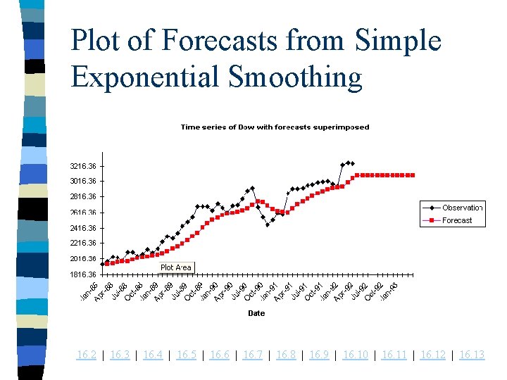
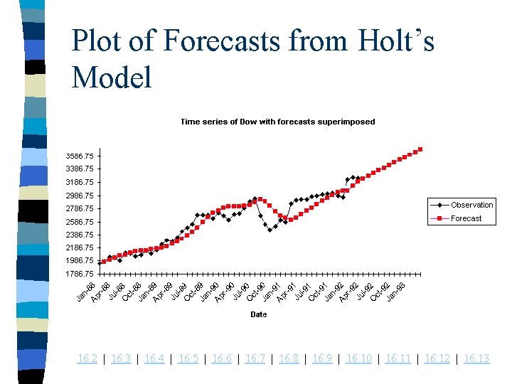
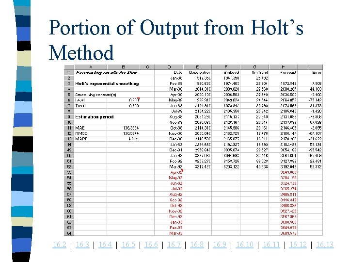
Solution n This first graph shows how a simple exponential smoothing model handles this trend, using alpha = 0. 2. n The graph’s summary error messages are not bad (MAPE is 5. 38%), but the forecasted series is obviously lagging behind the original series. n Also, the forecasts for the next 12 months are constant, because no trend is built into the model. n In contrast, the following graph shows forecasts from Holt’s model with alpha = beta = 0. 2. The forecasts are still far from perfect (MAPE is now 4. 01%), but at least the upward trend has been captured 16. 2 | 16. 3 | 16. 4 | 16. 5 | 16. 6 | 16. 7 | 16. 8 | 16. 9 | 16. 10 | 16. 11 | 16. 12 | 16. 13

Plot of Forecasts from Simple Exponential Smoothing 16. 2 | 16. 3 | 16. 4 | 16. 5 | 16. 6 | 16. 7 | 16. 8 | 16. 9 | 16. 10 | 16. 11 | 16. 12 | 16. 13

Plot of Forecasts from Holt’s Model 16. 2 | 16. 3 | 16. 4 | 16. 5 | 16. 6 | 16. 7 | 16. 8 | 16. 9 | 16. 10 | 16. 11 | 16. 12 | 16. 13

Holt’s Method n The exponential smoothing method generally works well if there is no obvious trend in the series. But if there is a trend, then this method lags behind. n Holt’s model rectifies this by dealing with trend explicitly. n Holt’s model includes a trend term and a corresponding smoothing constant. This new smoothing constant (beta) controls how quickly the method reacts to perceived changes in the trend. 16. 2 | 16. 3 | 16. 4 | 16. 5 | 16. 6 | 16. 7 | 16. 8 | 16. 9 | 16. 10 | 16. 11 | 16. 12 | 16. 13

Using Holt’s Method n To produce the output from Holt’s method with Stat. Pro we proceed exactly as with the simple exponential procedure. The only difference is that we now get to choose two smoothing parameters. n The output is also very similar to simple exponential smoothing output, except that there is now an extra column (column G) for the estimated trend. 16. 2 | 16. 3 | 16. 4 | 16. 5 | 16. 6 | 16. 7 | 16. 8 | 16. 9 | 16. 10 | 16. 11 | 16. 12 | 16. 13

Portion of Output from Holt’s Method 16. 2 | 16. 3 | 16. 4 | 16. 5 | 16. 6 | 16. 7 | 16. 8 | 16. 9 | 16. 10 | 16. 11 | 16. 12 | 16. 13

Smoothing Constants n It was mentioned that the smoothing constants used above are not optimal. n If we use an Stat. Pro’s optimize option to find the best alpha for simple exponential smoothing or the best alpha and beta for the Holt’s method. n In this case we find 1. 0 and 0. 0 for the smoothing constants. n Therefore, the best forecast for next month’s value is the month’s value plus a constant trend. 16. 2 | 16. 3 | 16. 4 | 16. 5 | 16. 6 | 16. 7 | 16. 8 | 16. 9 | 16. 10 | 16. 11 | 16. 12 | 16. 13

Exponential Smoothing

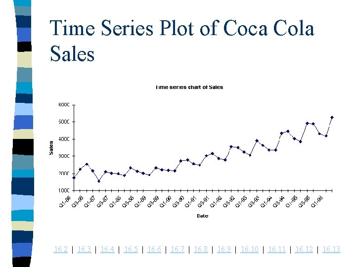
COCACOLA. XLS n The data in this spreadsheet represents quarterly sales for Coca Cola from the first quarter of 1986 through the second quarter of 1996. n As we might expect there has been an upward trend in sales during this period and there is also a fairly regular seasonal pattern as shown in the time series plot of sales. n Sales in warmer quarters, 2 and 3, are consistently higher than in the colder quarters, 1 and 4. n How well can Winter’s method track this upward tend and seasonal pattern? 16. 2 | 16. 3 | 16. 4 | 16. 5 | 16. 6 | 16. 7 | 16. 8 | 16. 9 | 16. 10 | 16. 11 | 16. 12 | 16. 13

Time Series Plot of Coca Cola Sales 16. 2 | 16. 3 | 16. 4 | 16. 5 | 16. 6 | 16. 7 | 16. 8 | 16. 9 | 16. 10 | 16. 11 | 16. 12 | 16. 13

Seasonality n Seasonality if defined as the consistent month-tomonth (or quarter-to-quarter) differences that occur each year. n The easiest way to check if there is seasonality in a time series is to look at a plot of the times series to see if it has a regular pattern of up and/or downs in particular months or quarters. n There are basically two extrapolation methods for dealing with seasonality: – We can use a model that takes seasonality into account or; – We can deseasonalize the data, forecast the data, and then adjust the forecasts for seasonality. 16. 2 | 16. 3 | 16. 4 | 16. 5 | 16. 6 | 16. 7 | 16. 8 | 16. 9 | 16. 10 | 16. 11 | 16. 12 | 16. 13

Seasonality -- continued n Winters’ model is of the first type. It attacks seasonality directly. n Seasonality models are usually classified as additive or multiplicative. – An additive model finds seasonal indexes, one for each month, that we add to the monthly average to get a particular month’s value. – A multiplicative model also finds seasonal indexes, but we multiply the monthly average by these indexes to get a particular month’s value. n Either model can be used but multiplicative models are somewhat easier to interpret. 16. 2 | 16. 3 | 16. 4 | 16. 5 | 16. 6 | 16. 7 | 16. 8 | 16. 9 | 16. 10 | 16. 11 | 16. 12 | 16. 13

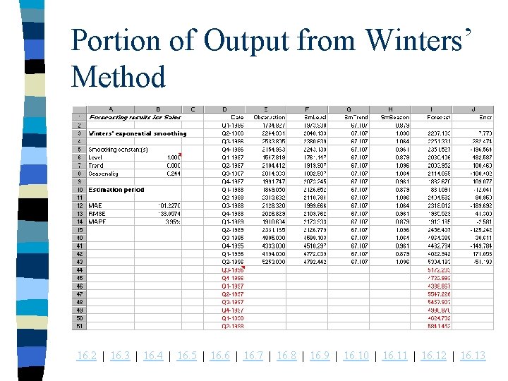
Winter’s Model of Seasonality n Winters’ model is very similar to Holt’s model - it has level and trend terms and corresponding smoothing constants alpha and beta - but it also has seasonal indexes and a corresponding smoothing constant. n The new smoothing constant controls how quickly the method reacts to perceived changes in the pattern of seasonality. n If the constant is small, the method reacts slowly; if the constant is large, it reacts more quickly. 16. 2 | 16. 3 | 16. 4 | 16. 5 | 16. 6 | 16. 7 | 16. 8 | 16. 9 | 16. 10 | 16. 11 | 16. 12 | 16. 13

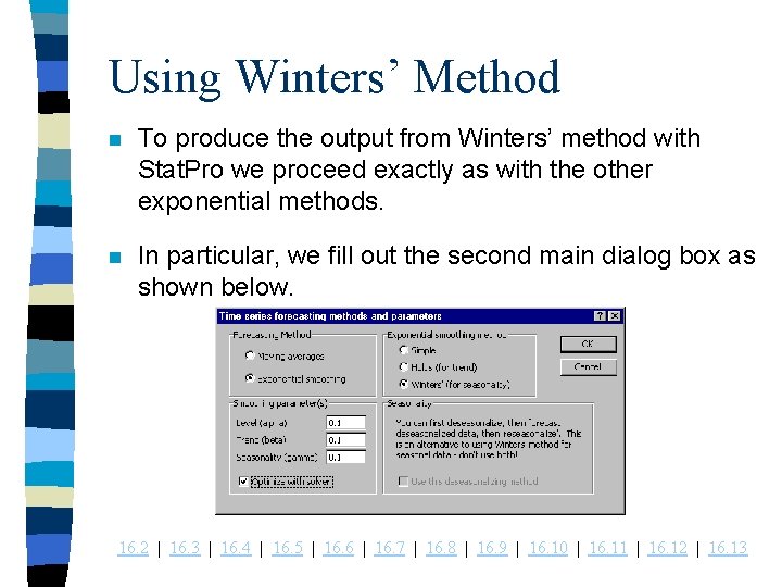
Using Winters’ Method n To produce the output from Winters’ method with Stat. Pro we proceed exactly as with the other exponential methods. n In particular, we fill out the second main dialog box as shown below. 16. 2 | 16. 3 | 16. 4 | 16. 5 | 16. 6 | 16. 7 | 16. 8 | 16. 9 | 16. 10 | 16. 11 | 16. 12 | 16. 13

Portion of Output from Winters’ Method 16. 2 | 16. 3 | 16. 4 | 16. 5 | 16. 6 | 16. 7 | 16. 8 | 16. 9 | 16. 10 | 16. 11 | 16. 12 | 16. 13

The Output n The optimal smoothing constants (those that minimize RMSE) are 1. 0, 0. 0 and 0. 244. Intuitively, these mean react right away to changes in level, never react to changes in trend, and react fairly slowly to changes in the seasonal pattern. n If we ignore seasonality, the series is trending upward at a rate of 67. 107 per quarter. n The seasonal pattern stays constant throughout this 10 -year period. n The forecast series tracks the actual series quite well. 16. 2 | 16. 3 | 16. 4 | 16. 5 | 16. 6 | 16. 7 | 16. 8 | 16. 9 | 16. 10 | 16. 11 | 16. 12 | 16. 13

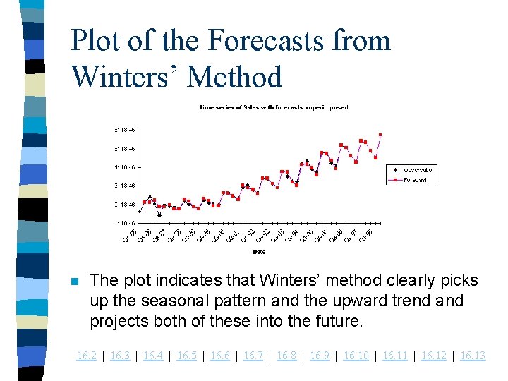
Plot of the Forecasts from Winters’ Method n The plot indicates that Winters’ method clearly picks up the seasonal pattern and the upward trend and projects both of these into the future. 16. 2 | 16. 3 | 16. 4 | 16. 5 | 16. 6 | 16. 7 | 16. 8 | 16. 9 | 16. 10 | 16. 11 | 16. 12 | 16. 13

In Conclusion n Some analysts would suggest using more “typical” values for the constants such as alpha=beta=0. 2 and 0. 5 for the seasonality constant. n To see how these smoothing constants would affect the results, we can simply substitute their values into the range B 6: B 8. n The summary measures get worse, yet the plot still indicates a very good fit. 16. 2 | 16. 3 | 16. 4 | 16. 5 | 16. 6 | 16. 7 | 16. 8 | 16. 9 | 16. 10 | 16. 11 | 16. 12 | 16. 13

Deseasonalizing: The Ratio-to-Moving-Averages Method

COCACOLA. XLS n We return to this data file that contains the sales history from 1986 to quarter 2 of 1996. n Is it possible to obtain the same forecast accuracy with the ratio-to-moving-averages method as we obtained with the Winters’ method? 16. 2 | 16. 3 | 16. 4 | 16. 5 | 16. 6 | 16. 7 | 16. 8 | 16. 9 | 16. 10 | 16. 11 | 16. 12 | 16. 13

Ratio-to-Moving-Averages Method n There are many varieties of sophisticated methods for deseasonalizing time series data but they are all variations of the ratio-to-moving-averages method. n This method is applicable when we believe that seasonality is multiplicative. n The goal is to find the seasonal indexes, which can then be used to deseasonalize the data. n The method is not meant for hand calculations and is straightforward to implement with Stat. Pro. 16. 2 | 16. 3 | 16. 4 | 16. 5 | 16. 6 | 16. 7 | 16. 8 | 16. 9 | 16. 10 | 16. 11 | 16. 12 | 16. 13

Solution n The answer to the question posed earlier depends on which forecasting method we use to forecast the deseasonalized data. n The ratio-to-moving-averages method only provides a means for deseasonalizing the data and providing seasonal indexes. Beyond this, any method can be used to forecast the deseasonalized data, and some methods work better than others. n For this example, we will compare two methods: the moving averages method with a span of 4 quarters, and Holt’s exponential smoothing method optimized. 16. 2 | 16. 3 | 16. 4 | 16. 5 | 16. 6 | 16. 7 | 16. 8 | 16. 9 | 16. 10 | 16. 11 | 16. 12 | 16. 13

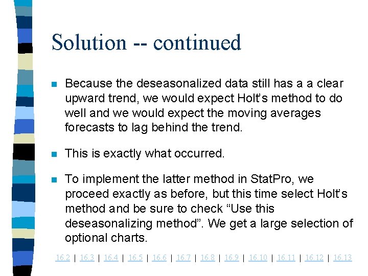
Solution -- continued n Because the deseasonalized data still has a a clear upward trend, we would expect Holt’s method to do well and we would expect the moving averages forecasts to lag behind the trend. n This is exactly what occurred. n To implement the latter method in Stat. Pro, we proceed exactly as before, but this time select Holt’s method and be sure to check “Use this deseasonalizing method”. We get a large selection of optional charts. 16. 2 | 16. 3 | 16. 4 | 16. 5 | 16. 6 | 16. 7 | 16. 8 | 16. 9 | 16. 10 | 16. 11 | 16. 12 | 16. 13

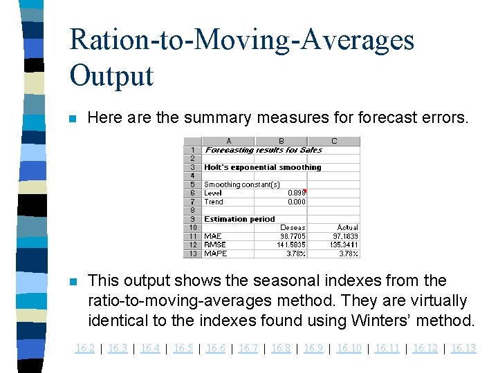
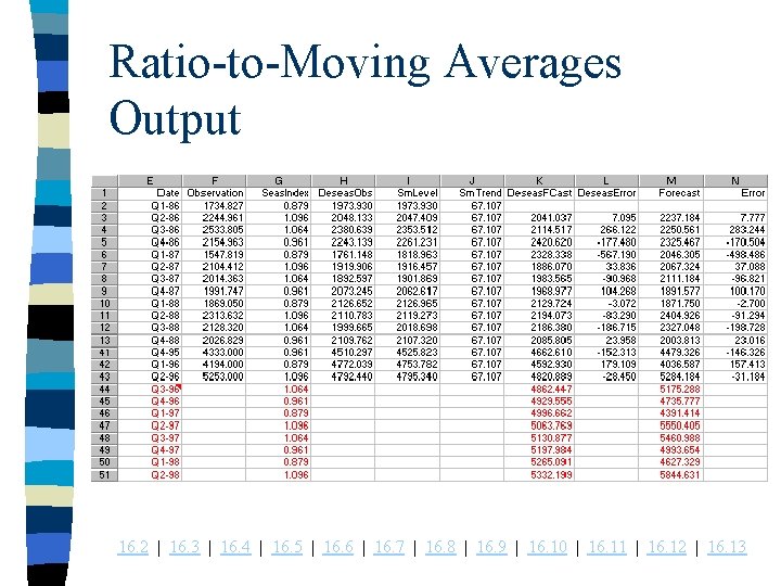
Ration-to-Moving-Averages Output n Here are the summary measures forecast errors. n This output shows the seasonal indexes from the ratio-to-moving-averages method. They are virtually identical to the indexes found using Winters’ method. 16. 2 | 16. 3 | 16. 4 | 16. 5 | 16. 6 | 16. 7 | 16. 8 | 16. 9 | 16. 10 | 16. 11 | 16. 12 | 16. 13

Ratio-to-Moving Averages Output 16. 2 | 16. 3 | 16. 4 | 16. 5 | 16. 6 | 16. 7 | 16. 8 | 16. 9 | 16. 10 | 16. 11 | 16. 12 | 16. 13

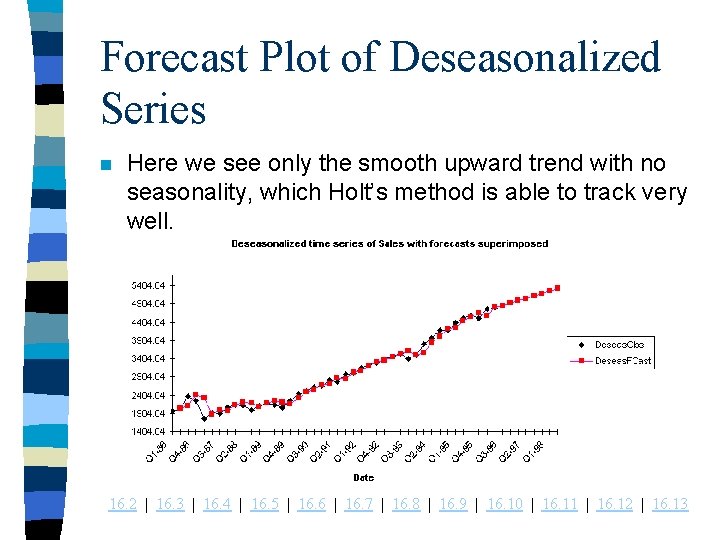
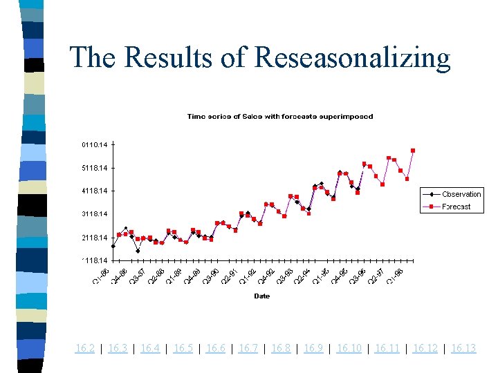
Forecast Plot of Deseasonalized Series n Here we see only the smooth upward trend with no seasonality, which Holt’s method is able to track very well. 16. 2 | 16. 3 | 16. 4 | 16. 5 | 16. 6 | 16. 7 | 16. 8 | 16. 9 | 16. 10 | 16. 11 | 16. 12 | 16. 13

The Results of Reseasonalizing 16. 2 | 16. 3 | 16. 4 | 16. 5 | 16. 6 | 16. 7 | 16. 8 | 16. 9 | 16. 10 | 16. 11 | 16. 12 | 16. 13

Summary Measures n The summary measures of forecast errors below are quite comparable to those from Winters’ method. n The reason is that both arrive at virtually the same seasonal pattern. 16. 2 | 16. 3 | 16. 4 | 16. 5 | 16. 6 | 16. 7 | 16. 8 | 16. 9 | 16. 10 | 16. 11 | 16. 12 | 16. 13

Estimating Seasonality with Regression

COCACOLA. XLS n We return to this data file which contains the sales history of Coca Cola from 1986 to quarter 2 of 1996. n Does a regression approach provide forecasts that are as accurate as those provided by the other seasonal methods in this chapter? 16. 2 | 16. 3 | 16. 4 | 16. 5 | 16. 6 | 16. 7 | 16. 8 | 16. 9 | 16. 10 | 16. 11 | 16. 12 | 16. 13

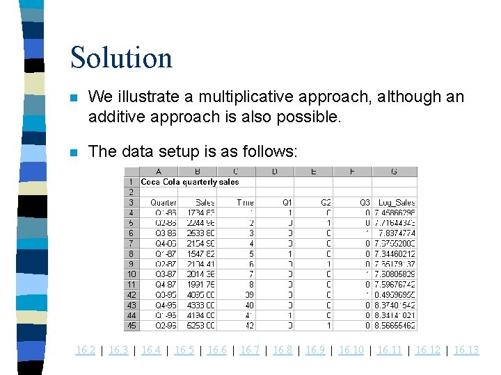
Solution n We illustrate a multiplicative approach, although an additive approach is also possible. n The data setup is as follows: 16. 2 | 16. 3 | 16. 4 | 16. 5 | 16. 6 | 16. 7 | 16. 8 | 16. 9 | 16. 10 | 16. 11 | 16. 12 | 16. 13

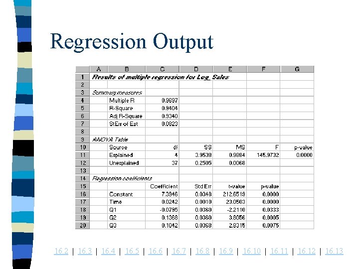
Solution n Besides the Sales and Time variables, we need dummy variables for three of the four quarters and a Log_Sales variable. n We then can use multiple regression, with the Log_sales as the response variable and Time, Q 1, Q 2, and Q 3 as the explanatory variables. n The regression output appears as follows: 16. 2 | 16. 3 | 16. 4 | 16. 5 | 16. 6 | 16. 7 | 16. 8 | 16. 9 | 16. 10 | 16. 11 | 16. 12 | 16. 13

Regression Output 16. 2 | 16. 3 | 16. 4 | 16. 5 | 16. 6 | 16. 7 | 16. 8 | 16. 9 | 16. 10 | 16. 11 | 16. 12 | 16. 13

Interpreting the Output n Of particular interest are the coefficients of the explanatory variables. n Recall that for a log response variable, these coefficients can be interpreted as percent changes in the original sales variable. n Specifically, the coefficient of Time means that deseasonalized sales increase by 2. 4% per quarter. n This pattern is quite comparable to the pattern of seasonal indexes we saw in the last two examples. 16. 2 | 16. 3 | 16. 4 | 16. 5 | 16. 6 | 16. 7 | 16. 8 | 16. 9 | 16. 10 | 16. 11 | 16. 12 | 16. 13

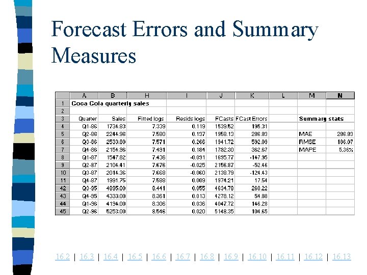
Forecast Accuracy n To compare the forecast accuracy of this method with earlier examples, we must go through several steps manually. – The multiple regression procedure in Stat. PRo provide fitted values and residuals for the log of sales. – We need to take these antilogs and obtain forecasts of the original sales data, and subtract these from the sales data to obtain forecast errors in Column K. – We can then use the formulas that were used in Stat. Pro’s forecasting procedure to obtain the summary measures MAE, RMSE, and MAPE. 16. 2 | 16. 3 | 16. 4 | 16. 5 | 16. 6 | 16. 7 | 16. 8 | 16. 9 | 16. 10 | 16. 11 | 16. 12 | 16. 13

Forecast Errors and Summary Measures 16. 2 | 16. 3 | 16. 4 | 16. 5 | 16. 6 | 16. 7 | 16. 8 | 16. 9 | 16. 10 | 16. 11 | 16. 12 | 16. 13

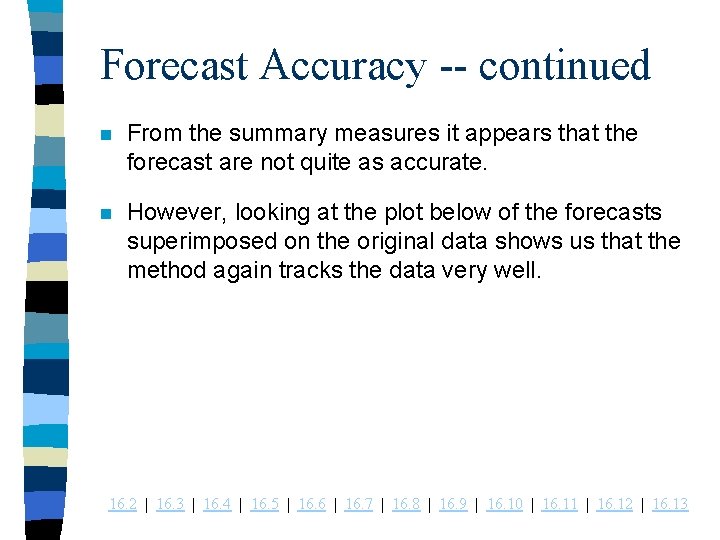
Forecast Accuracy -- continued n From the summary measures it appears that the forecast are not quite as accurate. n However, looking at the plot below of the forecasts superimposed on the original data shows us that the method again tracks the data very well. 16. 2 | 16. 3 | 16. 4 | 16. 5 | 16. 6 | 16. 7 | 16. 8 | 16. 9 | 16. 10 | 16. 11 | 16. 12 | 16. 13