Time Series Analysis TIME SERIES ANALYSIS Introduction Time

Time Series Analysis

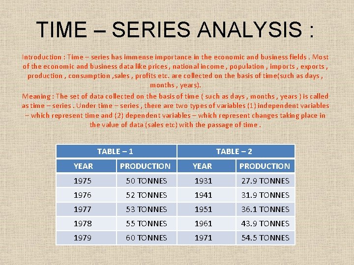
TIME – SERIES ANALYSIS : Introduction : Time – series has immense importance in the economic and business fields. Most of the economic and business data like prices , national income , population , imports , exports , production , consumption , sales , profits etc. are collected on the basis of time(such as days , months , years). Meaning : The set of data collected on the basis of time ( such as days , months , years ) is called as time – series. Under time – series , there are two types of variables (1) independent variables – which represent time and (2) dependent variables – which represent changes taking place in the value of data (sales etc) with the passage of time. TABLE – 1 TABLE – 2 YEAR PRODUCTION 1975 50 TONNES 1931 27. 9 TONNES 1976 52 TONNES 1941 31. 9 TONNES 1977 53 TONNES 1951 36. 1 TONNES 1978 55 TONNES 1961 43. 9 TONNES 1979 60 TONNES 1971 54. 5 TONNES

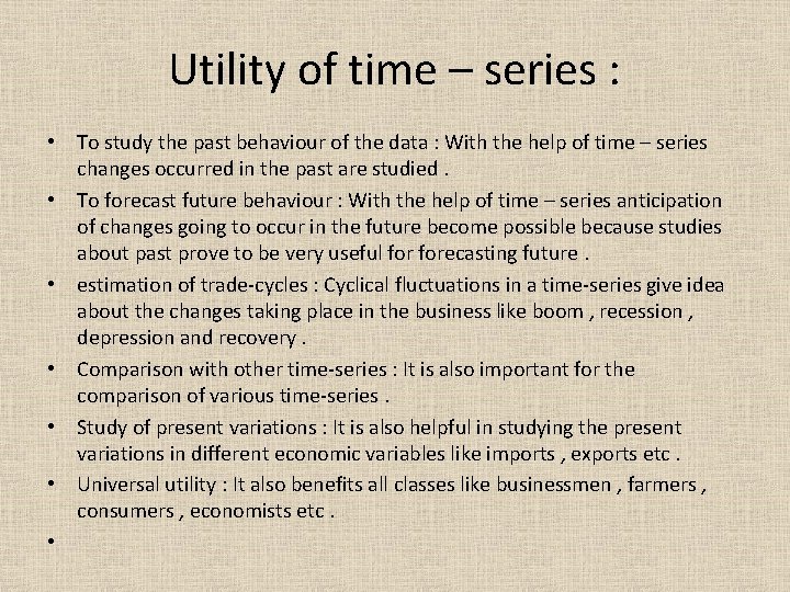
Utility of time – series : • To study the past behaviour of the data : With the help of time – series changes occurred in the past are studied. • To forecast future behaviour : With the help of time – series anticipation of changes going to occur in the future become possible because studies about past prove to be very useful forecasting future. • estimation of trade-cycles : Cyclical fluctuations in a time-series give idea about the changes taking place in the business like boom , recession , depression and recovery. • Comparison with other time-series : It is also important for the comparison of various time-series. • Study of present variations : It is also helpful in studying the present variations in different economic variables like imports , exports etc. • Universal utility : It also benefits all classes like businessmen , farmers , consumers , economists etc. •

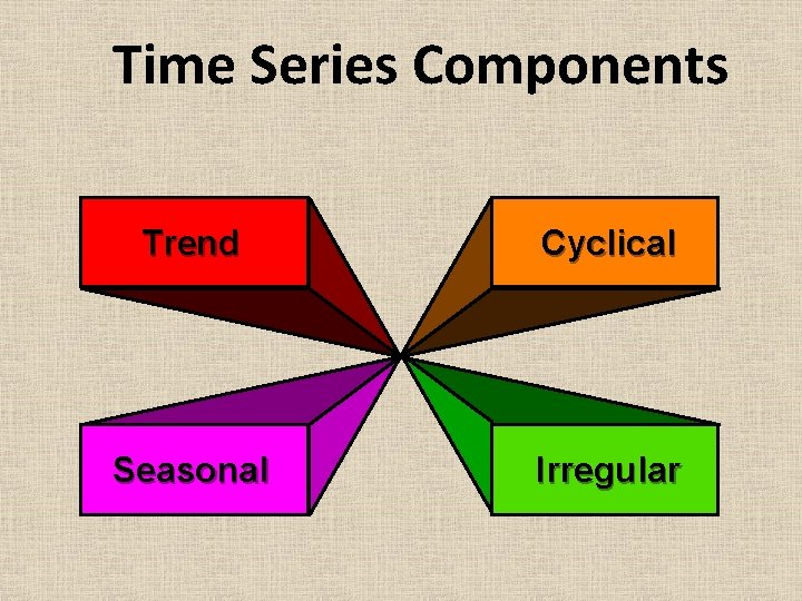
Time Series Components Trend Cyclical Seasonal Irregular

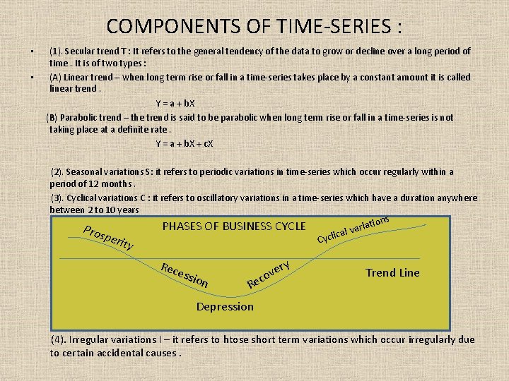
COMPONENTS OF TIME-SERIES : • • (1). Secular trend T : It refers to the general tendency of the data to grow or decline over a long period of time. It is of two types : (A) Linear trend – when long term rise or fall in a time-series takes place by a constant amount it is called linear trend. Y = a + b. X (B) Parabolic trend – the trend is said to be parabolic when long term rise or fall in a time-series is not taking place at a definite rate. Y = a + b. X + c. X (2). Seasonal variations S: it refers to periodic variations in time-series which occur regularly within a period of 12 months. (3). Cyclical variations C : it refers to oscillatory variations in a time-series which have a duration anywhere between 2 to 10 years Pros peri PHASES OF BUSINESS CYCLE ty Rec essi on y Re r e v co ions t a i r l va ca Cycli Trend Line Depression (4). Irregular variations I – it refers to htose short term variations which occur irregularly due to certain accidental causes.

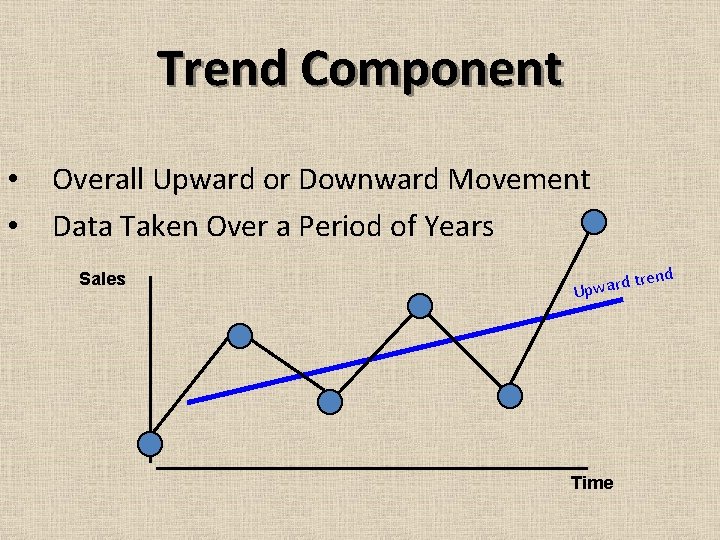
Trend Component • • Overall Upward or Downward Movement Data Taken Over a Period of Years Sales d Upwar Time trend

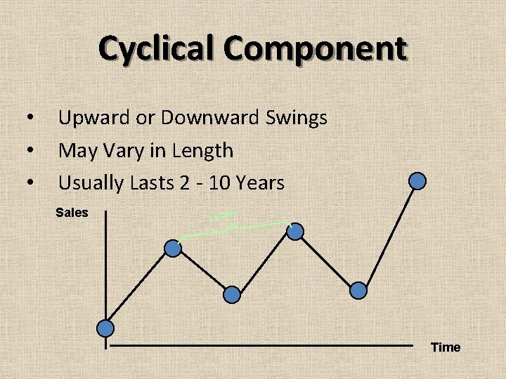
Cyclical Component • • • Upward or Downward Swings May Vary in Length Usually Lasts 2 - 10 Years Sales Cycle Time

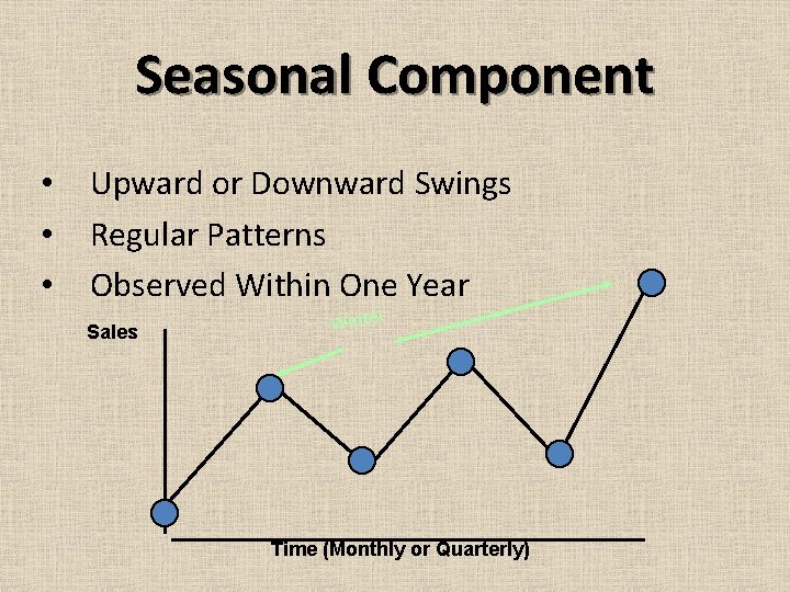
Seasonal Component • • • Upward or Downward Swings Regular Patterns Observed Within One Year Sales Winter Time (Monthly or Quarterly)

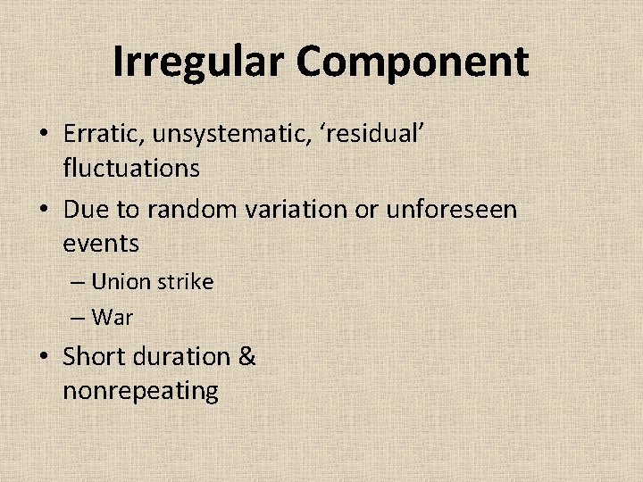
Irregular Component • Erratic, unsystematic, ‘residual’ fluctuations • Due to random variation or unforeseen events – Union strike – War • Short duration & nonrepeating

Random or Irregular Component • Erratic, Nonsystematic, Random, ‘Residual’ Fluctuations • Due to Random Variations of – Nature – Accidents • Short Duration and Non-repeating

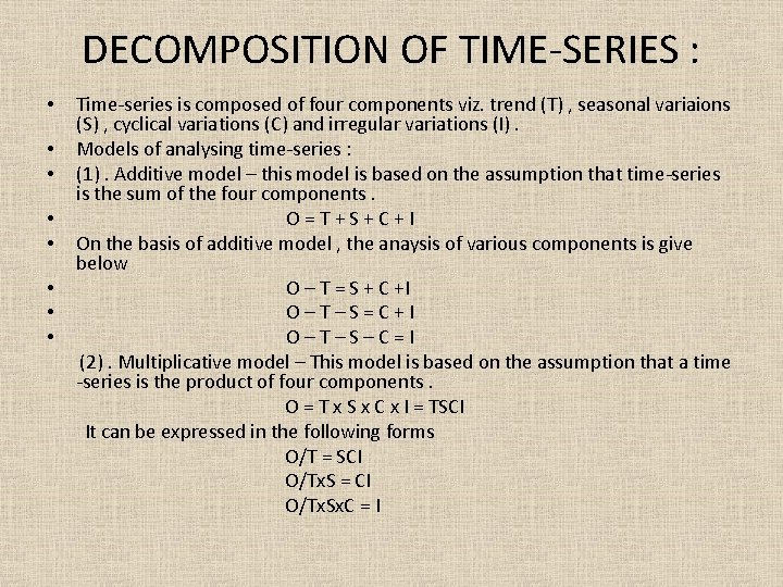
DECOMPOSITION OF TIME-SERIES : • • Time-series is composed of four components viz. trend (T) , seasonal variaions (S) , cyclical variations (C) and irregular variations (I). Models of analysing time-series : (1). Additive model – this model is based on the assumption that time-series is the sum of the four components. O=T+S+C+I On the basis of additive model , the anaysis of various components is give below O – T = S + C +I O–T–S=C+I O–T–S–C=I (2). Multiplicative model – This model is based on the assumption that a time -series is the product of four components. O = T x S x C x I = TSCI It can be expressed in the following forms O/T = SCI O/Tx. S = CI O/Tx. Sx. C = I

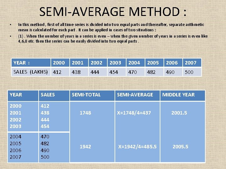
SEMI-AVERAGE METHOD : • • In this method , first of all time-series is divided into two equal parts and thereafter, separate arithmetic mean is calculated for each part. It can be applied in cases of two situations : (1). When the number of years in a series is even – when the given number of years in a series is even like 4, 6, 8 etc. then the series can be easily divided into two equal parts. YEAR : 2000 SALES (LAKHS) 412 YEAR SALES 2000 2001 2002 2003 412 438 444 454 2005 2006 2007 470 482 490 500 2001 2002 2003 2004 2005 2006 2007 438 444 454 470 482 490 500 SEMI-TOTAL SEMI-AVERAGE MIDDLE YEAR 1748 X=1748/4=437 2001. 5 1942 X=1942/4=485. 5 2005. 5

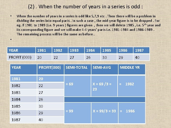
(2). When the number of years in a series is odd : • When the number of years in a series is odd like 5, 7, 9 etc. Then there will be a problem in dividing the series into equal parts. In such a case , the mid-year figure is to be dropped. For eg. If 1981 to 1989 (i. e. 9 years ) figures are given , then we will delete 1985 , i. e. 5 th year and its corresponding figure and we will make 4 -4 years’ parts i. e. 1981 -1984 and 1986 -1989. The remaining process will be the same as before. • YEAR 1981 1982 1983 1984 1985 1986 1987 PROFIT (000) 20 22 27 26 30 29 40 YEAR PROFIT(000) 1981 20 1982 22 1983 27 1984 26 1985 30 1986 29 1987 40 SEMI-TOTAL SEMI-AVG MIDDLE YR = 69 X = 69 /3 = 23 = 1982 = 99 X = 99/3 = 33 = 1986

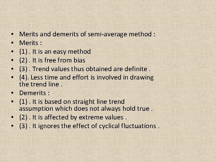
• • • Merits and demerits of semi-average method : Merits : (1). It is an easy method (2). It is free from bias (3). Trend values thus obtained are definite. (4). Less time and effort is involved in drawing the trend line. Demerits : (1). It is based on straight line trend assumption which does not always hold true. (2). It is affected by extreme values. (3). It ignores the effect of cyclical fluctuations.

Moving Average Method

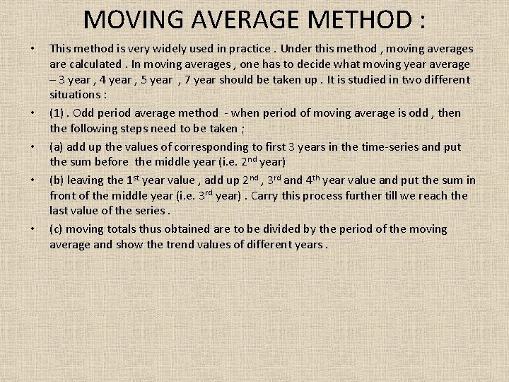
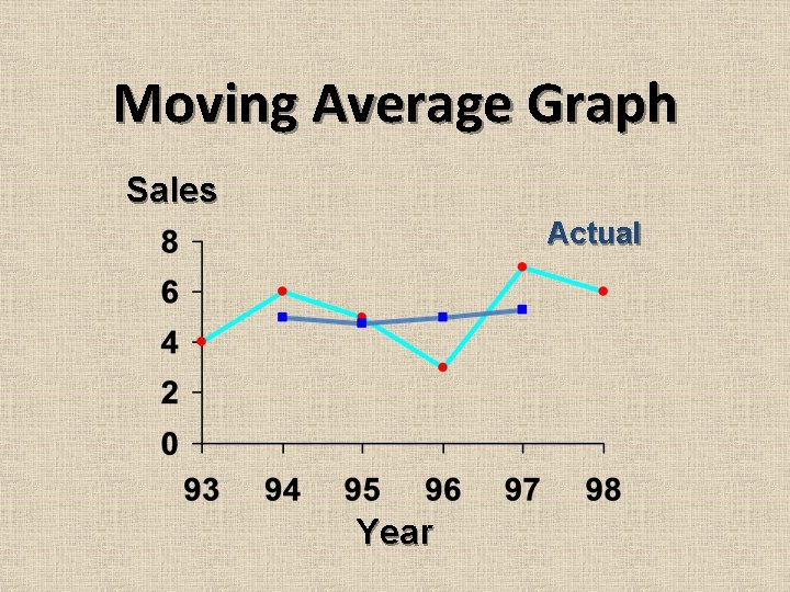
MOVING AVERAGE METHOD : • • • This method is very widely used in practice. Under this method , moving averages are calculated. In moving averages , one has to decide what moving year average – 3 year , 4 year , 5 year , 7 year should be taken up. It is studied in two different situations : (1). Odd period average method - when period of moving average is odd , then the following steps need to be taken ; (a) add up the values of corresponding to first 3 years in the time-series and put the sum before the middle year (i. e. 2 nd year) (b) leaving the 1 st year value , add up 2 nd , 3 rd and 4 th year value and put the sum in front of the middle year (i. e. 3 rd year). Carry this process further till we reach the last value of the series. (c) moving totals thus obtained are to be divided by the period of the moving average and show the trend values of different years.

Moving Average Graph Sales Actual Year

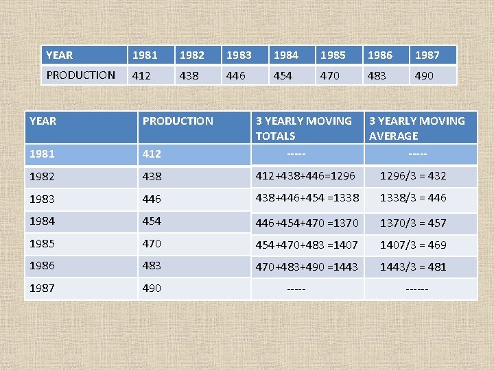
YEAR 1981 1982 1983 1984 1985 1986 1987 PRODUCTION 412 438 446 454 470 483 490 YEAR PRODUCTION 412 3 YEARLY MOVING TOTALS ----- 3 YEARLY MOVING AVERAGE ----- 1981 19 1982 438 412+438+446=1296/3 = 432 1983 446 438+446+454 =1338/3 = 446 1984 454 446+454+470 =1370/3 = 457 1985 470 454+470+483 =1407/3 = 469 1986 483 470+483+490 =1443/3 = 481 1987 490 ------

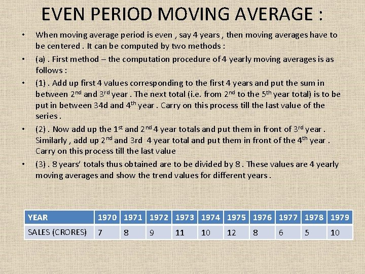
EVEN PERIOD MOVING AVERAGE : • • • When moving average period is even , say 4 years , then moving averages have to be centered. It can be computed by two methods : (a). First method – the computation procedure of 4 yearly moving averages is as follows : (1). Add up first 4 values corresponding to the first 4 years and put the sum in between 2 nd and 3 rd year. The next total (i. e. from 2 nd to the 5 th year total) is to be put in between 34 d and 4 th year. Carry on this process till the last value of the series. (2). Now add up the 1 st and 2 nd 4 year totals and put them in front of 3 rd year. Similarly , add up 2 nd and 3 rd 4 year total and put them in front of the 4 th year. Carry on this process till the last value (3). 8 years’ totals thus obtained are to be divided by 8. These values are 4 yearly moving averages and show the trend values for different years. YEAR 1970 1971 1972 1973 1974 1975 1976 1977 1978 1979 SALES (CRORES) 7 8 9 11 10 12 8 6 5 10

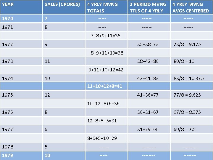
YEAR SALES (CRORES) 7 4 YRLY MVNG TOTALS ----- 2 PERIOD MVNG TTLS OF 4 YRLY ------ 1970 1971 4 YRLY MVNG AVGS CENTERED ------ 8 ------ 35+38=73 73/8 = 9. 125 38+42=80 80/8 = 10 42+41=83 83/8 = 10. 375 41+36=77 77/8 = 9. 625 36+31=67 67/8 = 8. 375 31+29=60 60/8 = 7. 5 7+8+9+11=35 1972 9 8+9+11+10=38 1973 11 9+11+10+12=42 1974 10 11+10+12+8=41 1975 12 10+12+8+6=36 1976 8 12+8+6+5=31 1977 6 8+6+5+10=29 1978 5 -------- 1979 10 --------

Freehand Curve Method

Freehand Curve [Graph] Production Actual Year

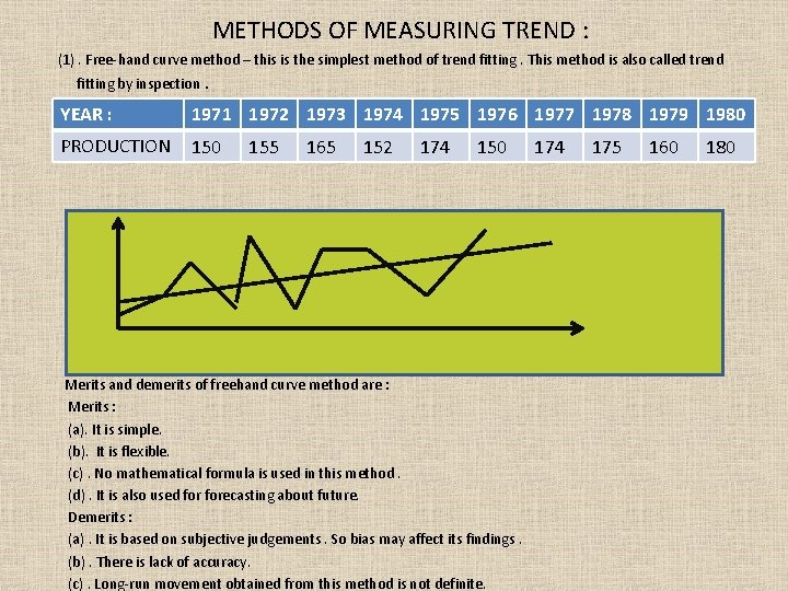
METHODS OF MEASURING TREND : (1). Free-hand curve method – this is the simplest method of trend fitting. This method is also called trend fitting by inspection. YEAR : 1971 1972 1973 1974 1975 1976 1977 1978 1979 1980 PRODUCTION 150 155 165 152 174 150 Merits and demerits of freehand curve method are : Merits : (a). It is simple. (b). It is flexible. (c). No mathematical formula is used in this method. (d). It is also used forecasting about future. Demerits : (a). It is based on subjective judgements. So bias may affect its findings. (b). There is lack of accuracy. (c). Long-run movement obtained from this method is not definite. 174 175 160 180

Least Square Method :

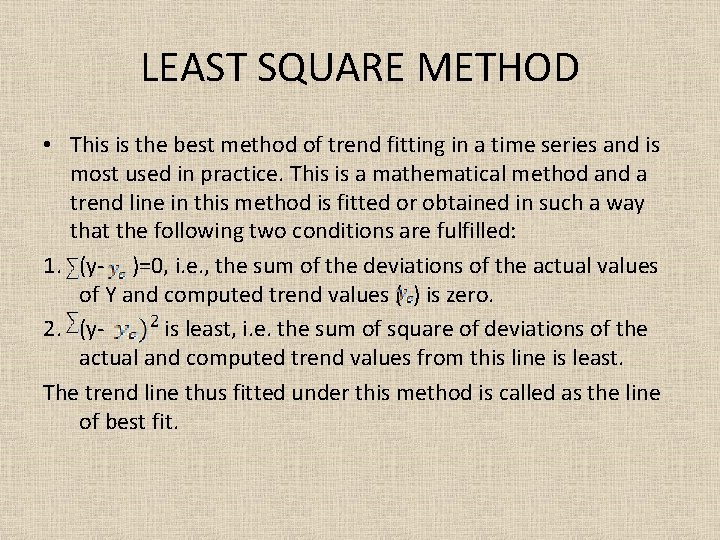
LEAST SQUARE METHOD • This is the best method of trend fitting in a time series and is most used in practice. This is a mathematical method and a trend line in this method is fitted or obtained in such a way that the following two conditions are fulfilled: 1. (y- )=0, i. e. , the sum of the deviations of the actual values of Y and computed trend values ( ) is zero. 2. (yis least, i. e. the sum of square of deviations of the actual and computed trend values from this line is least. The trend line thus fitted under this method is called as the line of best fit.

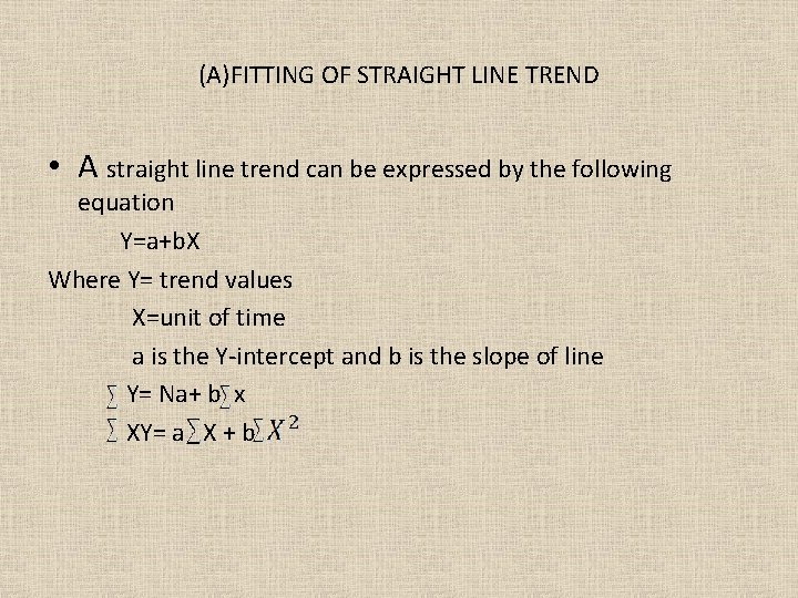
(A)FITTING OF STRAIGHT LINE TREND • A straight line trend can be expressed by the following equation Y=a+b. X Where Y= trend values X=unit of time a is the Y-intercept and b is the slope of line Y= Na+ b x XY= a X + b

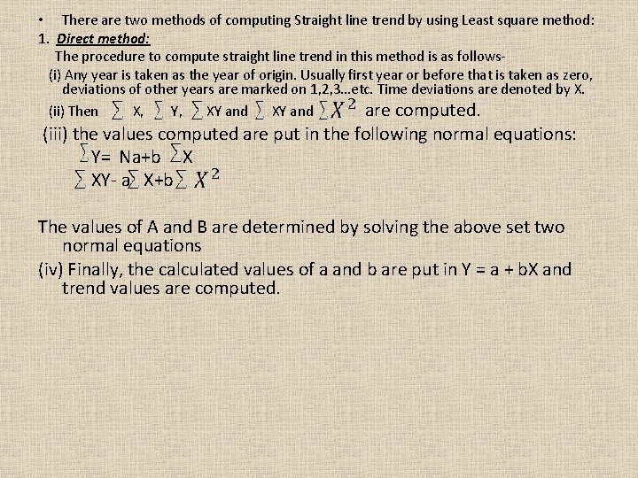
• There are two methods of computing Straight line trend by using Least square method: 1. Direct method: The procedure to compute straight line trend in this method is as follows(i) Any year is taken as the year of origin. Usually first year or before that is taken as zero, deviations of other years are marked on 1, 2, 3…etc. Time deviations are denoted by X. (ii) Then X, Y, XY and are computed. (iii) the values computed are put in the following normal equations: Y= Na+b X XY- a X+b The values of A and B are determined by solving the above set two normal equations (iv) Finally, the calculated values of a and b are put in Y = a + b. X and trend values are computed.

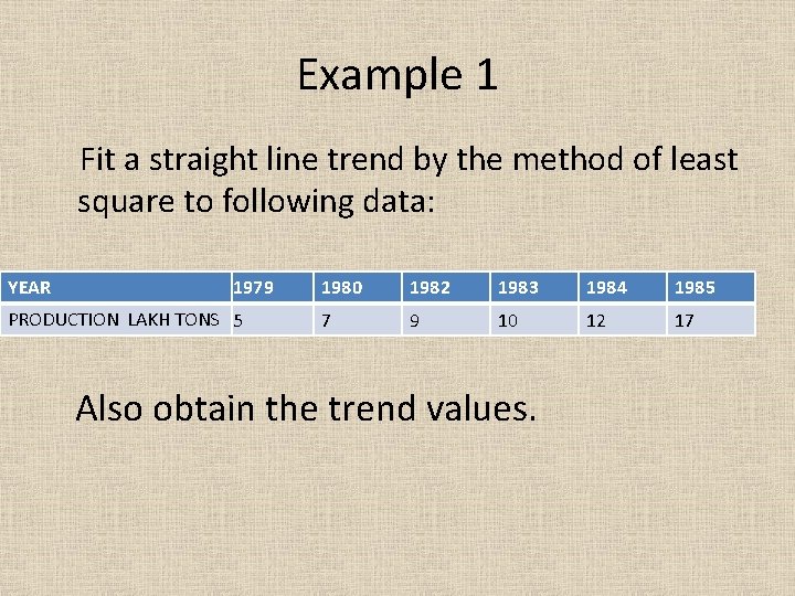
Example 1 Fit a straight line trend by the method of least square to following data: YEAR 1979 PRODUCTION LAKH TONS 5 1980 1982 1983 1984 1985 7 9 10 12 17 Also obtain the trend values.

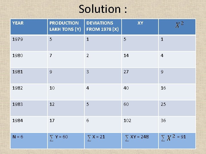
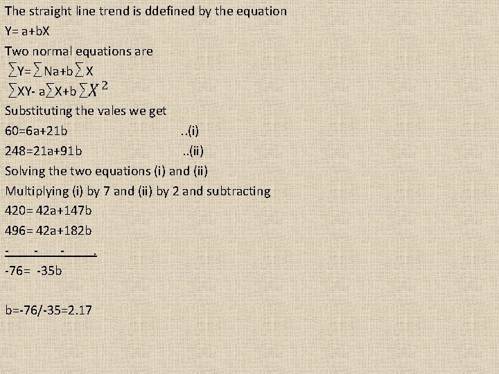
Solution : YEAR PRODUCTION LAKH TONS (Y) DEVIATIONS FROM 1978 (X) 1979 5 1 1980 7 2 14 4 1981 9 3 27 9 1982 10 4 40 16 1983 12 5 60 25 1984 17 6 102 36 N=6 Y = 60 X = 21 XY XY = 248 = 91

The straight line trend is ddefined by the equation Y= a+b. X Two normal equations are Y= Na+b X XY- a X+b Substituting the vales we get 60=6 a+21 b. . (i) 248=21 a+91 b. . (ii) Solving the two equations (i) and (ii) Multiplying (i) by 7 and (ii) by 2 and subtracting 420= 42 a+147 b 496= 42 a+182 b. -76= -35 b b=-76/-35=2. 17

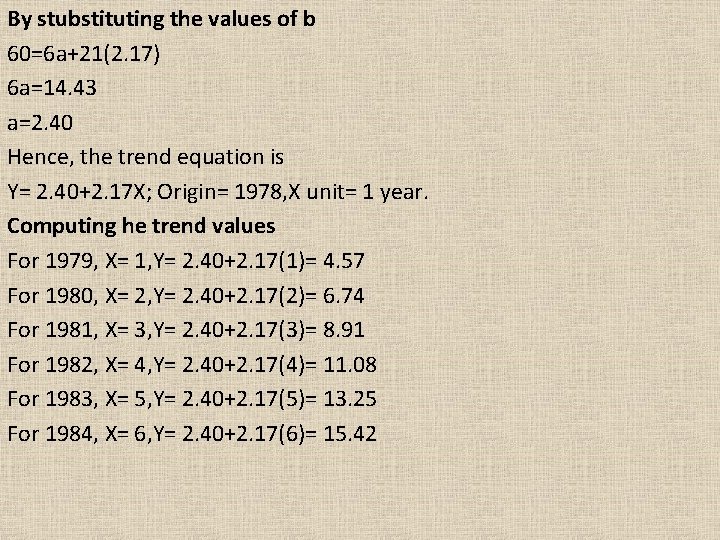
By stubstituting the values of b 60=6 a+21(2. 17) 6 a=14. 43 a=2. 40 Hence, the trend equation is Y= 2. 40+2. 17 X; Origin= 1978, X unit= 1 year. Computing he trend values For 1979, X= 1, Y= 2. 40+2. 17(1)= 4. 57 For 1980, X= 2, Y= 2. 40+2. 17(2)= 6. 74 For 1981, X= 3, Y= 2. 40+2. 17(3)= 8. 91 For 1982, X= 4, Y= 2. 40+2. 17(4)= 11. 08 For 1983, X= 5, Y= 2. 40+2. 17(5)= 13. 25 For 1984, X= 6, Y= 2. 40+2. 17(6)= 15. 42

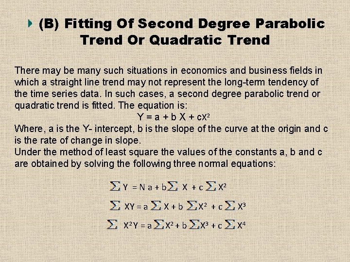
(B) Fitting Of Second Degree Parabolic Trend Or Quadratic Trend There may be many such situations in economics and business fields in which a straight line trend may not represent the long-term tendency of the time series data. In such cases, a second degree parabolic trend or quadratic trend is fitted. The equation is: Y = a + b X + c. X 2 Where, a is the Y- intercept, b is the slope of the curve at the origin and c is the rate of change in slope. Under the method of least square the values of the constants a, b and c are obtained by solving the following three normal equations: Y =Na+b X +c X 2 XY = a X+b X 2 + c X 3 X 2 Y = a X 2 + b X 3 + c X 4

SHORTCUT METHOD

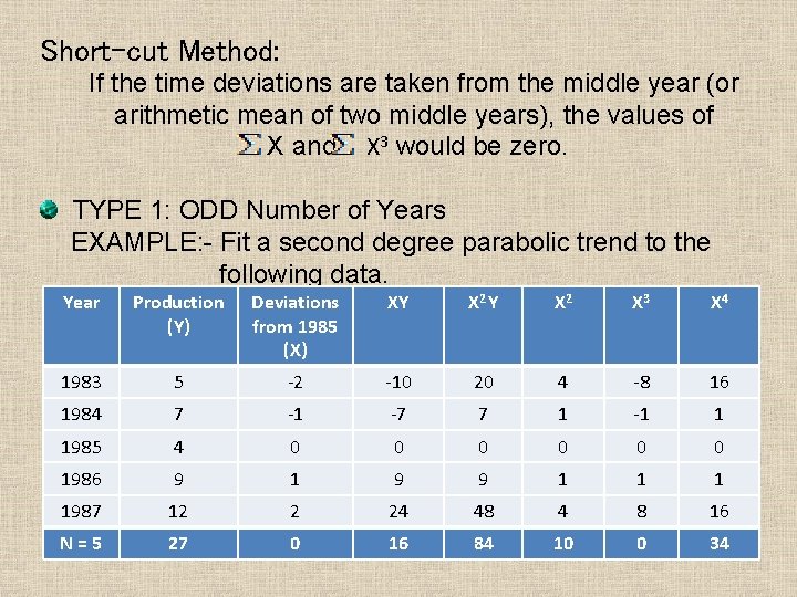
Short-cut Method: If the time deviations are taken from the middle year (or arithmetic mean of two middle years), the values of X and X 3 would be zero. TYPE 1: ODD Number of Years EXAMPLE: - Fit a second degree parabolic trend to the following data. Year Production (Y) Deviations from 1985 (X) XY X 2 X 3 X 4 1983 5 -2 -10 20 4 -8 16 1984 7 -1 -7 7 1 -1 1 1985 4 0 0 0 1986 9 1 9 9 1 1987 12 2 24 48 4 8 16 N=5 27 0 16 84 10 0 34

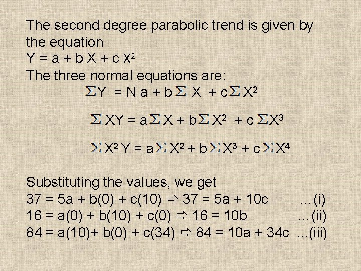
The second degree parabolic trend is given by the equation Y = a + b X + c X 2 The three normal equations are: Y = N a + b X + c X 2 XY = a X 2 Y = a X+b X 2 + c X 3 X 4 Substituting the values, we get 37 = 5 a + b(0) + c(10) 37 = 5 a + 10 c …(i) 16 = a(0) + b(10) + c(0) 16 = 10 b …(ii) 84 = a(10)+ b(0) + c(34) 84 = 10 a + 34 c. . . (iii)

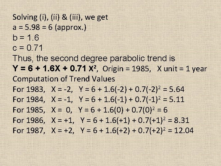
Solving (i), (ii) & (iii), we get a = 5. 98 = 6 (approx. ) b = 1. 6 c = 0. 71 Thus, the second degree parabolic trend is Y = 6 + 1. 6 X + 0. 71 X 2, Origin = 1985, X unit = 1 year Computation of Trend Values For 1983, X = -2, Y = 6 + 1. 6(-2) + 0. 7(-2)2 = 5. 64 For 1984, X = -1, Y = 6 + 1. 6(-1) + 0. 7(-1)2 = 5. 11 For 1985, X = 0, Y = 6 + 1. 6(0) + 0. 7(0)2 = 6 For 1986, X = +1, Y = 6 + 1. 6(+1) + 0. 7(+1)2 = 8. 31 For 1987, X = +2, Y = 6 + 1. 6(+2) + 0. 7(+2)2 = 12. 04

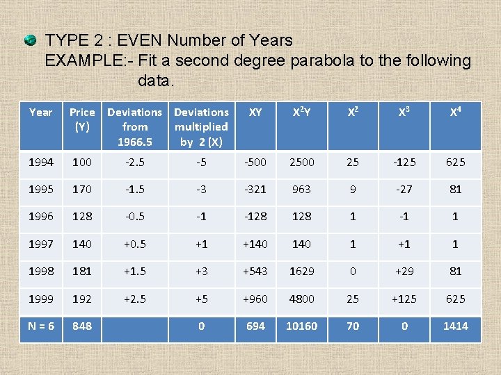
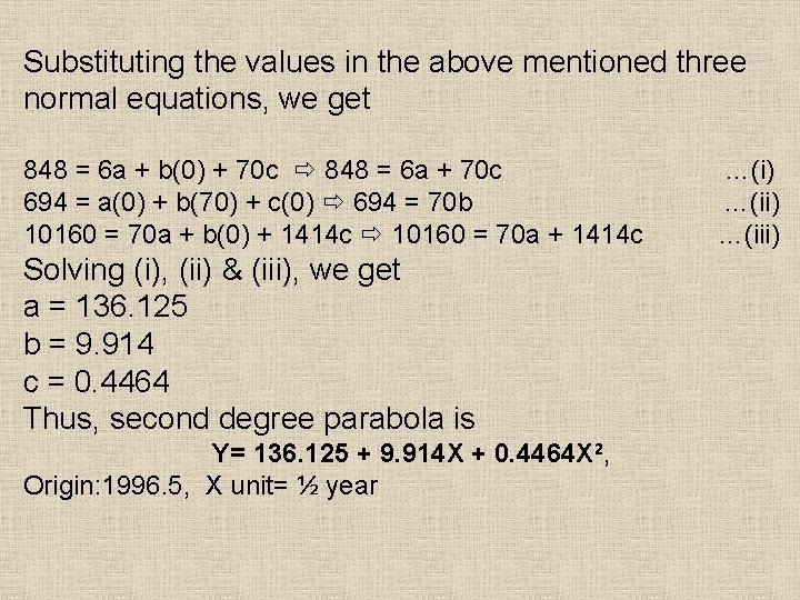
TYPE 2 : EVEN Number of Years EXAMPLE: - Fit a second degree parabola to the following data. Year Price Deviations (Y) from multiplied 1966. 5 by 2 (X) XY X 2 X 3 X 4 1994 100 -2. 5 -5 -500 25 -125 625 1995 170 -1. 5 -3 -321 963 9 -27 81 1996 128 -0. 5 -1 -128 1 -1 1 1997 140 +0. 5 +1 +140 1 +1 1 1998 181 +1. 5 +3 +543 1629 0 +29 81 1999 192 +2. 5 +5 +960 4800 25 +125 625 N=6 848 0 694 10160 70 0 1414

Substituting the values in the above mentioned three normal equations, we get 848 = 6 a + b(0) + 70 c 848 = 6 a + 70 c 694 = a(0) + b(70) + c(0) 694 = 70 b 10160 = 70 a + b(0) + 1414 c 10160 = 70 a + 1414 c Solving (i), (ii) & (iii), we get a = 136. 125 b = 9. 914 c = 0. 4464 Thus, second degree parabola is Y= 136. 125 + 9. 914 X + 0. 4464 X 2, Origin: 1996. 5, X unit= ½ year …(i) …(iii)

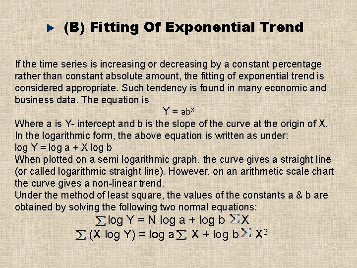
(B) Fitting Of Exponential Trend If the time series is increasing or decreasing by a constant percentage rather than constant absolute amount, the fitting of exponential trend is considered appropriate. Such tendency is found in many economic and business data. The equation is Y = ab. X Where a is Y- intercept and b is the slope of the curve at the origin of X. In the logarithmic form, the above equation is written as under: log Y = log a + X log b When plotted on a semi logarithmic graph, the curve gives a straight line (or called logarithmic straight line). However, on an arithmetic scale chart the curve gives a non-linear trend. Under the method of least square, the values of the constants a & b are obtained by solving the following two normal equations: log Y = N log a + log b X (X log Y) = log a X + log b X 2

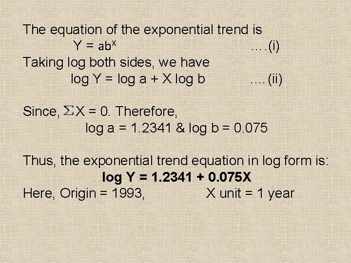
The equation of the exponential trend is Y = ab. X …. (i) Taking log both sides, we have log Y = log a + X log b. …(ii) Since, X = 0. Therefore, log a = 1. 2341 & log b = 0. 075 Thus, the exponential trend equation in log form is: log Y = 1. 2341 + 0. 075 X Here, Origin = 1993, X unit = 1 year

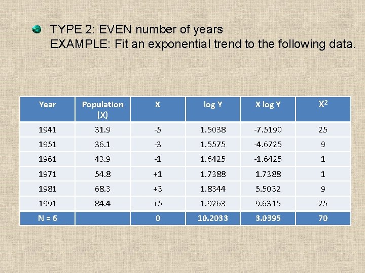
TYPE 2: EVEN number of years EXAMPLE: Fit an exponential trend to the following data. Year Population (X) X log Y X 2 1941 31. 9 -5 1. 5038 -7. 5190 25 1951 36. 1 -3 1. 5575 -4. 6725 9 1961 43. 9 -1 1. 6425 -1. 6425 1 1971 54. 8 +1 1. 7388 1 1981 68. 3 +3 1. 8344 5. 5032 9 1991 84. 4 +5 1. 9263 9. 6315 25 0 10. 2033 3. 0395 70 N=6

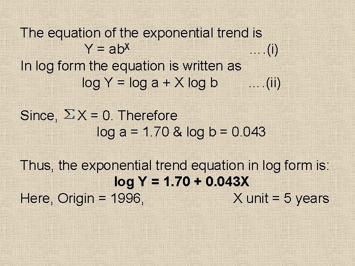
The equation of the exponential trend is Y = ab. X …. (i) In log form the equation is written as log Y = log a + X log b …. (ii) Since, X = 0. Therefore log a = 1. 70 & log b = 0. 043 Thus, the exponential trend equation in log form is: log Y = 1. 70 + 0. 043 X Here, Origin = 1996, X unit = 5 years

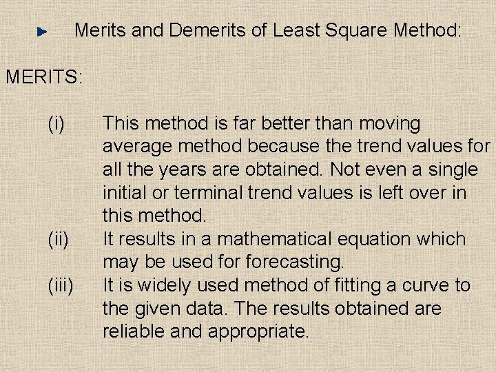
Merits and Demerits of Least Square Method: MERITS: (i) (iii) This method is far better than moving average method because the trend values for all the years are obtained. Not even a single initial or terminal trend values is left over in this method. It results in a mathematical equation which may be used forecasting. It is widely used method of fitting a curve to the given data. The results obtained are reliable and appropriate.

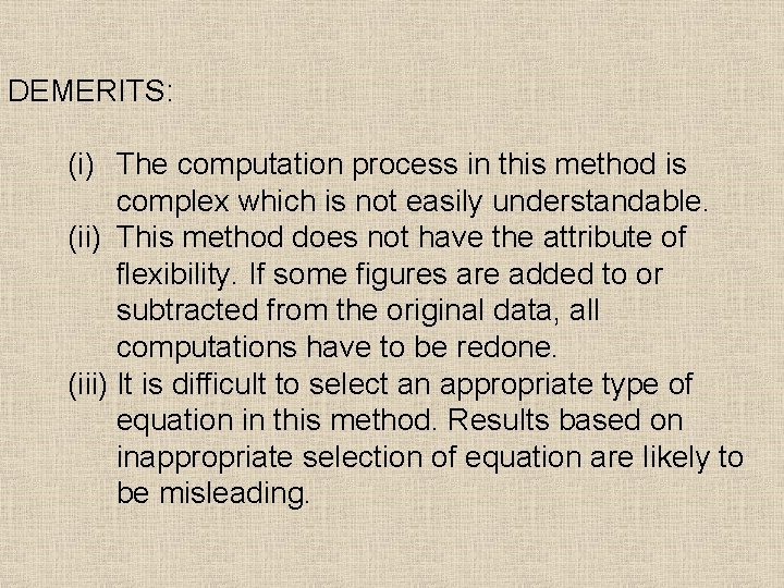
DEMERITS: (i) The computation process in this method is complex which is not easily understandable. (ii) This method does not have the attribute of flexibility. If some figures are added to or subtracted from the original data, all computations have to be redone. (iii) It is difficult to select an appropriate type of equation in this method. Results based on inappropriate selection of equation are likely to be misleading.