Time Series Analysis Demand Forecasting Page 1 A

Time Series Analysis (Demand Forecasting) Page 1

• A time series is a set of numerical values of a given variable listed at successive intervals of time, which means that, data regarding the variables is listed in chronological order. Usually the interval of time taken is uniform. • For example, yearly production of wheat in a country, hourly temperature of a city, monthly electricity bill of a flat etc. Page 2

Relevance of Time Series • In 1990 s, the US Govt. was much concerned about the problem of pollution in the country. • The US Environmental Protection Agency (EPA) monitored the quality of the air around the country based on time period yearly. • While data is provided about the content of the pollutants, the major question before experts were : a. Is it possible to forecast the future content of the pollutants based on the past years data? b. What can be the best forecasting method? § The above questions can be answered easily with the help of Time Series Analysis. Page 3

TIME SERIES ANALYSIS • If the time series is given, we can study about the forces that influence the variations in time series and the behavior of phenomenon over the given period of time. • For example, if sales data is given for a product for the period from 2005 to 2012, we will be able to say what can be the sales trend during 2013, 2014 etc. Even we will be able to say why sales has been less during certain period and why it has increased during certain other periods. • This implies that the forecaster is able to say why the values of the variable (sales) varies over period. Page 4

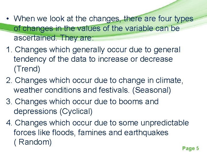
• When we look at the changes, there are four types of changes in the values of the variable can be ascertained. They are: 1. Changes which generally occur due to general tendency of the data to increase or decrease (Trend) 2. Changes which occur due to change in climate, weather conditions and festivals. (Seasonal) 3. Changes which occur due to booms and depressions (Cyclical) 4. Changes which occur due to some unpredictable forces like floods, famines and earthquakes ( Random) Page 5

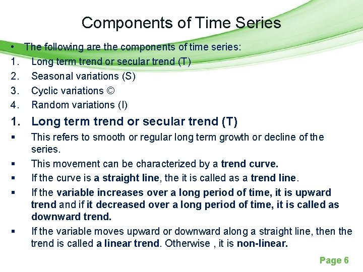
Components of Time Series • The following are the components of time series: 1. Long term trend or secular trend (T) 2. Seasonal variations (S) 3. Cyclic variations © 4. Random variations (I) 1. Long term trend or secular trend (T) § § § This refers to smooth or regular long term growth or decline of the series. This movement can be characterized by a trend curve. If the curve is a straight line, the it is called as a trend line. If the variable increases over a long period of time, it is upward trend and if it decreased over a long period of time, it is called as downward trend. If the variable moves upward or downward along a straight line, then the trend is called a linear trend. Otherwise , it is non-linear. Page 6

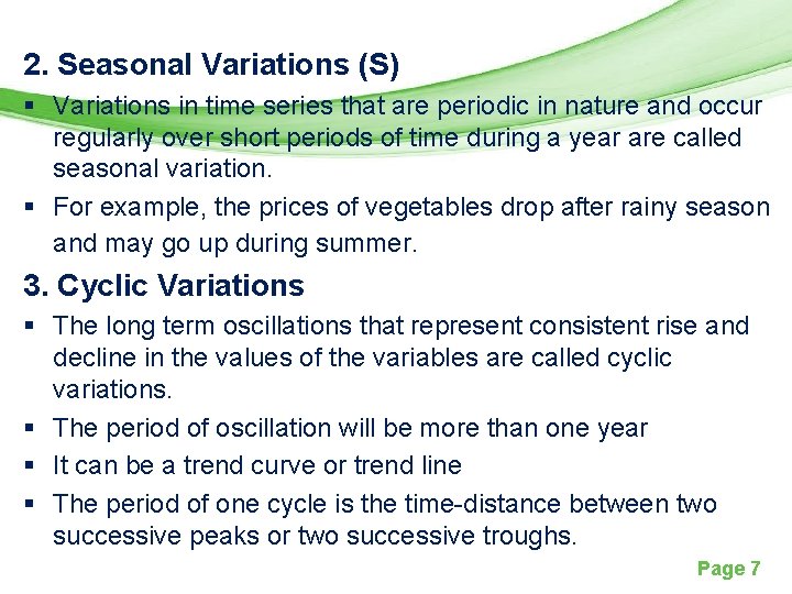
2. Seasonal Variations (S) § Variations in time series that are periodic in nature and occur regularly over short periods of time during a year are called seasonal variation. § For example, the prices of vegetables drop after rainy season and may go up during summer. 3. Cyclic Variations § The long term oscillations that represent consistent rise and decline in the values of the variables are called cyclic variations. § The period of oscillation will be more than one year § It can be a trend curve or trend line § The period of one cycle is the time-distance between two successive peaks or two successive troughs. Page 7

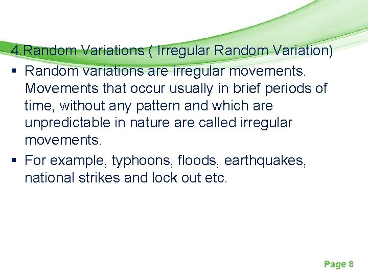
4. Random Variations ( Irregular Random Variation) § Random variations are irregular movements. Movements that occur usually in brief periods of time, without any pattern and which are unpredictable in nature are called irregular movements. § For example, typhoons, floods, earthquakes, national strikes and lock out etc. Page 8

METHODS OF MEASURING TREND • Trend can be measure by the following methods: 1. Free Hand or Graphic Method 2. Semi-Average Method 3. Moving Average Method 4. Method of Least Squares Page 9

1. Free Hand or Graphic Method • This is the simplest method of drawing a trend curve. • Plot the values of the variable against time on a graph paper and join these points. • Then the trend line will be drawn in such a way that the numbers of fluctuations on either side are approximately the same. The trend line will be a smooth curve. • Disadvantages of Free Hand Method § Depends on individual judgment § Cannot be used for predicting the trend as the drawing is arbitrary. Page 10

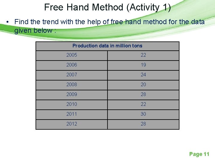
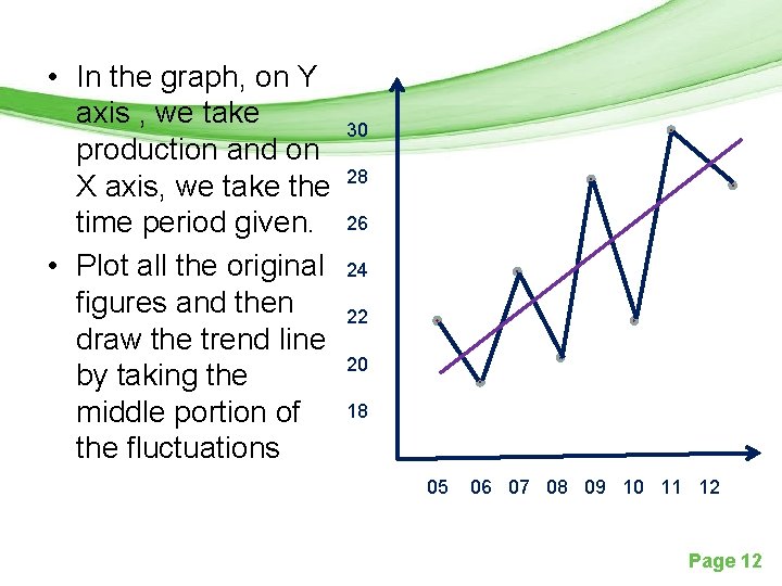
Free Hand Method (Activity 1) • Find the trend with the help of free hand method for the data given below : Production data in million tons 2005 22 2006 19 2007 24 2008 20 2009 28 2010 22 2011 30 2012 28 Page 11

• In the graph, on Y axis , we take production and on X axis, we take the time period given. • Plot all the original figures and then draw the trend line by taking the middle portion of the fluctuations 30 28 26 24 22 20 18 05 06 07 08 09 10 11 12 Page 12

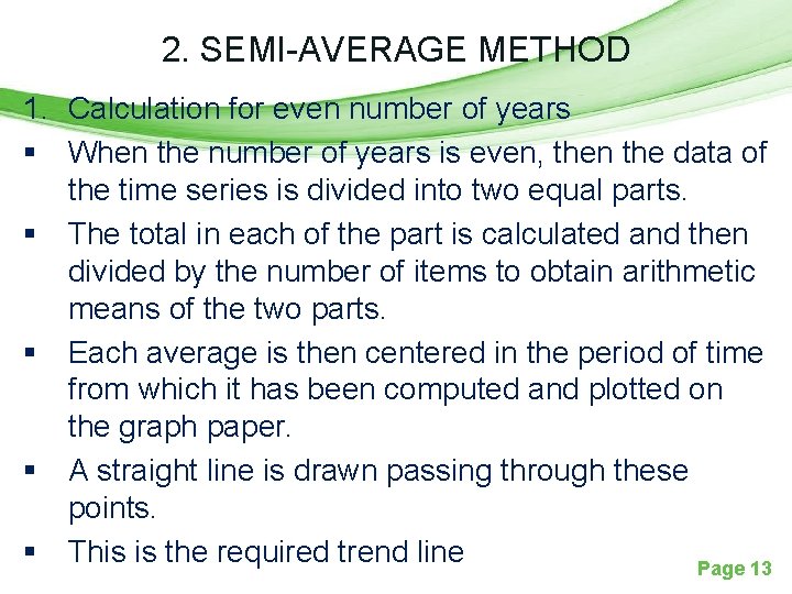
2. SEMI-AVERAGE METHOD 1. Calculation for even number of years § When the number of years is even, then the data of the time series is divided into two equal parts. § The total in each of the part is calculated and then divided by the number of items to obtain arithmetic means of the two parts. § Each average is then centered in the period of time from which it has been computed and plotted on the graph paper. § A straight line is drawn passing through these points. § This is the required trend line Page 13

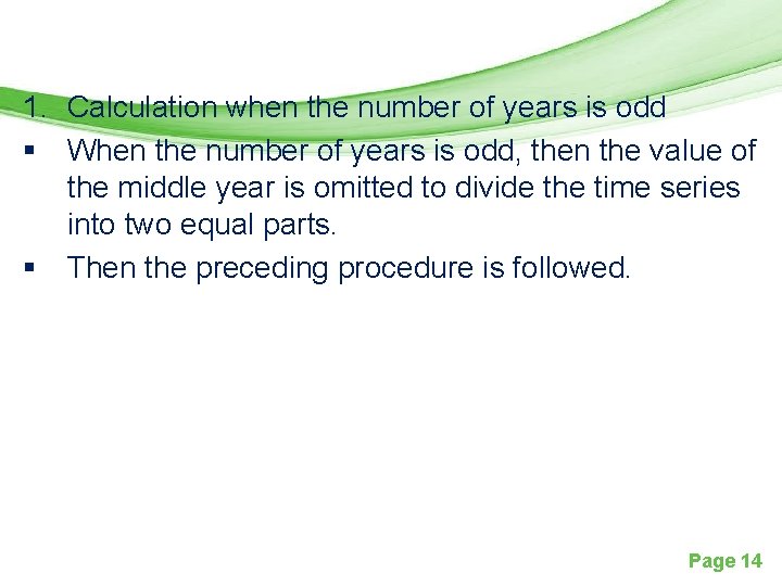
1. Calculation when the number of years is odd § When the number of years is odd, then the value of the middle year is omitted to divide the time series into two equal parts. § Then the preceding procedure is followed. Page 14

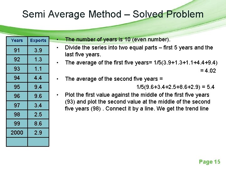
Semi Average Method – Solved Problem Years Exports 91 3. 9 92 1. 3 93 1. 1 94 4. 4 95 9. 4 96 9. 6 97 3. 4 98 2. 5 99 8. 6 2000 2. 9 • • • The number of years is 10 (even number). Divide the series into two equal parts – first 5 years and the last five years. The average of the first five years= 1/5(3. 9+1. 3+1. 1+4. 4+9. 4) = 4. 02 The average of the second five years = 1/5(9. 6+3. 4+2. 5+8. 6+2. 9) = 5. 4 Plot the first value against the middle of the first five years (93) and plot the second value at the middle of the second five years (98). Connect it by a line. We get the trend line Page 15

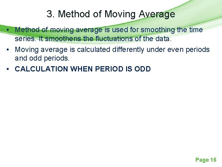
3. Method of Moving Average • Method of moving average is used for smoothing the time series. It smoothens the fluctuations of the data. • Moving average is calculated differently under even periods and odd periods. • CALCULATION WHEN PERIOD IS ODD Page 16

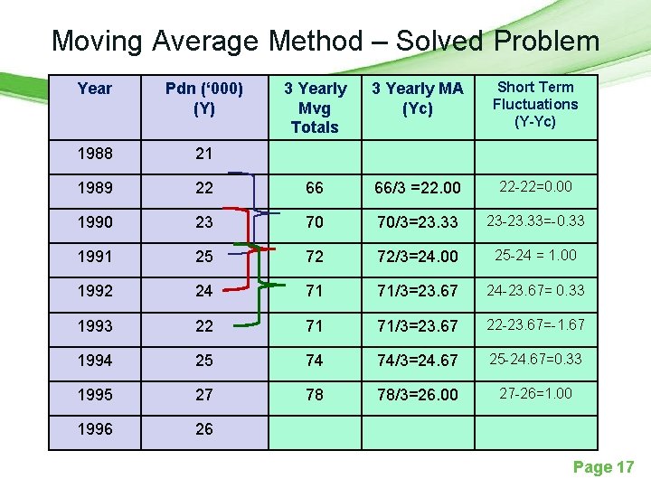
Moving Average Method – Solved Problem 3 Yearly Mvg Totals 3 Yearly MA (Yc) Short Term Fluctuations (Y-Yc) 22 66 66/3 =22. 00 22 -22=0. 00 1990 23 70 70/3=23. 33 23 -23. 33=-0. 33 1991 25 72 72/3=24. 00 25 -24 = 1. 00 1992 24 71 71/3=23. 67 24 -23. 67= 0. 33 1993 22 71 71/3=23. 67 22 -23. 67=-1. 67 1994 25 74 74/3=24. 67 25 -24. 67=0. 33 1995 27 78 78/3=26. 00 27 -26=1. 00 1996 26 Year Pdn (‘ 000) (Y) 1988 21 1989 Page 17

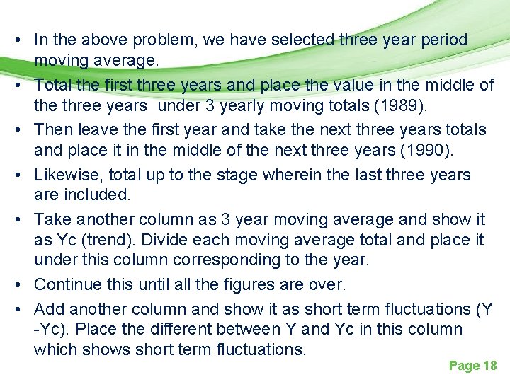
• In the above problem, we have selected three year period moving average. • Total the first three years and place the value in the middle of the three years under 3 yearly moving totals (1989). • Then leave the first year and take the next three years totals and place it in the middle of the next three years (1990). • Likewise, total up to the stage wherein the last three years are included. • Take another column as 3 year moving average and show it as Yc (trend). Divide each moving average total and place it under this column corresponding to the year. • Continue this until all the figures are over. • Add another column and show it as short term fluctuations (Y -Yc). Place the different between Y and Yc in this column which shows short term fluctuations. Page 18

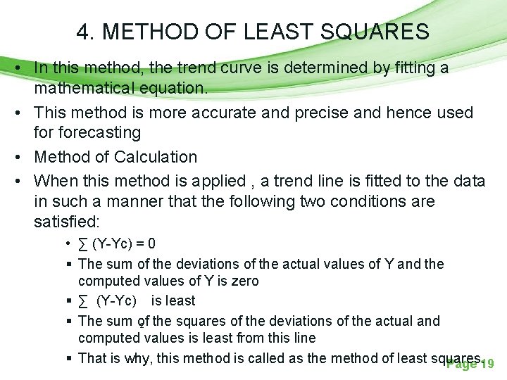
4. METHOD OF LEAST SQUARES • In this method, the trend curve is determined by fitting a mathematical equation. • This method is more accurate and precise and hence used forecasting • Method of Calculation • When this method is applied , a trend line is fitted to the data in such a manner that the following two conditions are satisfied: • ∑ (Y-Yc) = 0 § The sum of the deviations of the actual values of Y and the computed values of Y is zero § ∑ (Y-Yc) is least § The sum of 2 the squares of the deviations of the actual and computed values is least from this line § That is why, this method is called as the method of least squares. Page 19

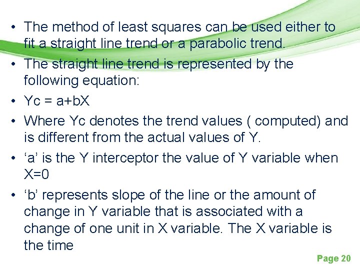
• The method of least squares can be used either to fit a straight line trend or a parabolic trend. • The straight line trend is represented by the following equation: • Yc = a+b. X • Where Yc denotes the trend values ( computed) and is different from the actual values of Y. • ‘a’ is the Y interceptor the value of Y variable when X=0 • ‘b’ represents slope of the line or the amount of change in Y variable that is associated with a change of one unit in X variable. The X variable is the time Page 20

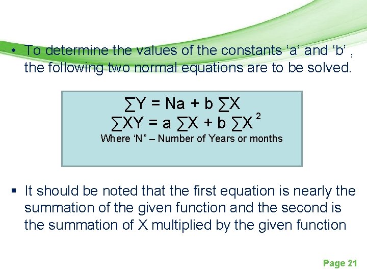
• To determine the values of the constants ‘a’ and ‘b’ , the following two normal equations are to be solved. ∑Y = Na + b ∑X 2 ∑XY = a ∑X + b ∑X Where ‘N” – Number of Years or months § It should be noted that the first equation is nearly the summation of the given function and the second is the summation of X multiplied by the given function Page 21

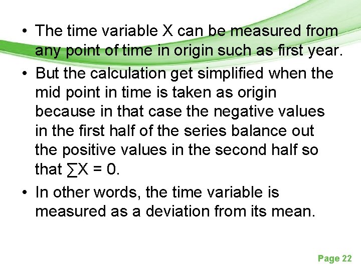
• The time variable X can be measured from any point of time in origin such as first year. • But the calculation get simplified when the mid point in time is taken as origin because in that case the negative values in the first half of the series balance out the positive values in the second half so that ∑X = 0. • In other words, the time variable is measured as a deviation from its mean. Page 22

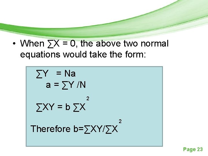
• When ∑X = 0, the above two normal equations would take the form: ∑Y = Na a = ∑Y /N 2 ∑XY = b ∑X Therefore b=∑XY/∑X 2 Page 23

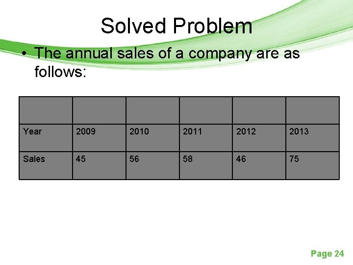
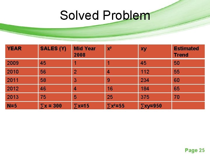
Solved Problem • The annual sales of a company are as follows: Year 2009 2010 2011 2012 2013 Sales 45 56 58 46 75 Page 24

Solved Problem YEAR SALES (Y) Mid Year 2008 x² xy Estimated Trend 2009 45 1 1 45 50 2010 56 2 4 112 55 2011 58 3 9 234 60 2012 46 4 16 184 65 2013 75 5 25 375 70 N=5 ∑x = 300 ∑x=15 ∑x²=55 ∑xy=950 Page 25

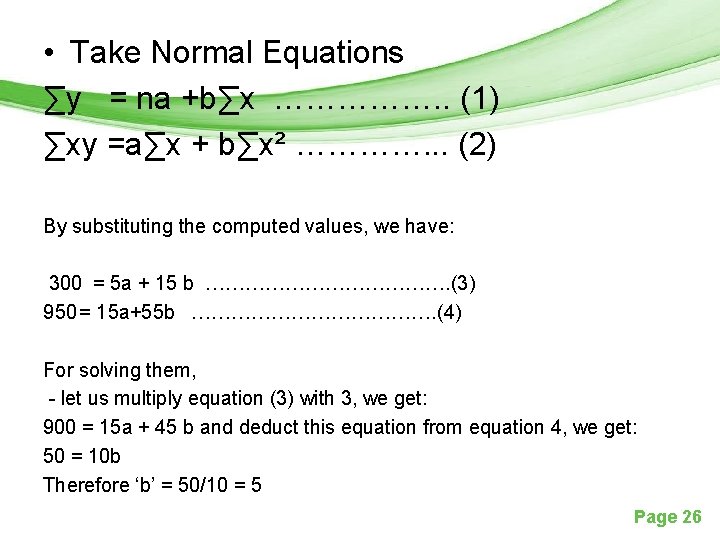
• Take Normal Equations ∑y = na +b∑x ……………. . (1) ∑xy =a∑x + b∑x² …………. . . (2) By substituting the computed values, we have: 300 = 5 a + 15 b ………………. (3) 950 = 15 a+55 b ………………. (4) For solving them, - let us multiply equation (3) with 3, we get: 900 = 15 a + 45 b and deduct this equation from equation 4, we get: 50 = 10 b Therefore ‘b’ = 50/10 = 5 Page 26

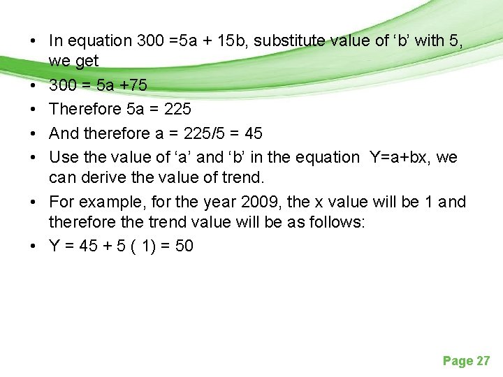
• In equation 300 =5 a + 15 b, substitute value of ‘b’ with 5, we get • 300 = 5 a +75 • Therefore 5 a = 225 • And therefore a = 225/5 = 45 • Use the value of ‘a’ and ‘b’ in the equation Y=a+bx, we can derive the value of trend. • For example, for the year 2009, the x value will be 1 and therefore the trend value will be as follows: • Y = 45 + 5 ( 1) = 50 Page 27

Mathematical Models in Time Series • The following are the two models: 1. Additive Model 2. Multiplicative Model Page 28

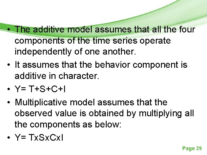
• The additive model assumes that all the four components of the time series operate independently of one another. • It assumes that the behavior component is additive in character. • Y= T+S+C+I • Multiplicative model assumes that the observed value is obtained by multiplying all the components as below: • Y= Tx. Sx. Cx. I Page 29

Mathematical Models in Time Series • The multiplicative model assumes that all the components are not necessarily independent and they can affect one another. • It also assumes that the behavior of the component is of multiplicative character. • All the values other than trend are rates or index numbers. Page 30

Measurement of Seasonal Variation • To derive the seasonal variations, we need to eliminate trend, cyclic variations and irregular fluctuations on the time series. • The main methods of measuring seasonal variations are: 1. Simple average method 2. Ratio to moving averages method 3. Chain or link relative method 4. Ratio to trend method Page 31