Time Frequency Analysis and Wavelet Transforms Office 723

Time Frequency Analysis and Wavelet Transforms 時頻分析與小波轉換 授課者： 丁 建 均 Office：明達館 723室, TEL： 33669652 E-mail: jjding@ntu. edu. tw 課程網頁：http: //djj. ee. ntu. edu. tw/TFW. htm 歡迎大家來修課，也歡迎有問題時隨時聯絡！ 1

5 上課時間： 17 週 9/14, 11/16, 出 HW 3 9/21, 11/23, 9/28 11/30, 交 HW 3 10/5, 出 HW 1 12/7, 出 HW 4 10/12, 12/14, Oral 10/19, 交 HW 1 12/2`, 10/26, 出 HW 2 12/28, 交 HW 4, 11/2, 1/4, 出 HW 5 11/9, 交 HW 2 1/18, 交 HW 5 及 term paper

6 課程大綱： (1) Introduction (2) Short-Time Fourier Transform (3) Gabor Transform (4) Implementation of Time-Frequency Analysis (5) Wigner Distribution Function (6) Cohen’s Class Time-Frequency Distribution (7) S Transforms, Gabor-Wigner Transforms, Matching Pursuit, and Other Time Frequency Analysis Methods (8) Movement in the Time-Frequency Plane and Fractional Fourier Transforms (9) Filter Design by Time-Frequency Analysis (10) Modulation, Multiplexing, Sampling, and Other Applications (續)

課程大綱： (11) Hilbert Huang Transform (12) From Haar Transforms to Wavelet Transforms (13) Continuous Wavelet Transforms (14) Continuous Wavelet Transform with Discrete Coefficients (15) Discrete Wavelet Transform (16) Applications of the Wavelet Transform 7

上課資料： (1) 講義 (將放在網頁上，請大家每次上課前先印好) (2) S. Qian and D. Chen, Joint Time-Frequency Analysis: Methods and Applications, Prentice-Hall, 1996. (3) L. Cohen, Time-Frequency Analysis, Prentice-Hall, New York, 1995. (4) K. Grochenig, Foundations of Time-Frequency Analysis, Birkhauser, Boston, 2001. (5) L. Debnath, Wavelet Transforms and Time-Frequency Signal Analysis, Birkhäuser, Boston, 2001. (6) S. Mallat, A Wavelet Tour of Signal Processing: The Sparse Way, Academic Press, 3 rd ed. , 2009. (7) Others 8

Tutorial 可供選擇的題目(可以略做修改) 有加 * 號的是學長寫過的，但鼓勵同學再加強 (1) Time-Frequency Reassignment (2) Sparse Time-Frequency Representation (3) Fast Algorithm for Time-Frequency Analysis (4) Time-Frequency Analysis for Machine Fault Detection (5) Orthogonal Matching Pursuit (6) Compressive Sensing for Signal Reconstruction (7) Compressive Sensing for Radar Imaging (8) Compressive Sensing for Communication (9) Compressive Sensing for Denoising (10) Hilbert-Huang Transform for EMG Signal Processing (11) Wavelet Transforms for Image Feature Extraction (12) Wavelet Transforms for Watermarking 10

I. Introduction Fourier transform (FT) Time-Domain Frequency Domain ↑ t varies from ∞~∞ Laplace Transform Cosine Transform, Sine Transform, Z Transform. Some things make these operations not practical: (1) Only the case where t 0 t t 1 is interested. (2) Not all the signals are suitable for analyzing in the frequency domain. It is hard to observe the variation of spectrum with time by these operations 11

12 Example 1: x(t) = cos(440 t) when t < 0. 5, x(t) = cos(660 t) when 0. 5 t < 1, x(t) = cos(524 t) when t 1 The Fourier transform of x(t) Frequency

13 (A) Finite-Supporting Fourier Transform (B) Short-Time Fourier Transform (STFT) w(t): window function 或 mask function STFT 也稱作 windowed Fourier transform 或 time-dependent Fourier transform [Ref] L. Cohen, Time-Frequency Analysis, Prentice-Hall, New York, 1995. [Ref] A. V. Oppenheim and R. W. Schafer, Discrete-Time Signal Processing, London: Prentice-Hall, 3 rd ed. , 2010.

14 最簡單的例子： w(t) = 1 for |t| B, -B B w(t) = 0 otherwise t-axis 此時 Short-time Fourier transform 可以改寫 其他的例子： 0 t-axis 一般我們把 exp(- σt 2) 稱作為 Gaussian function 或 Gabor function 此時的 Short-Time Fourier Transform 亦稱作 Gabor Transform

(C) Gabor Transform S. Qian and D. Chen, Joint Time-Frequency Analysis: Methods and Applications, Prentice Hall, N. J. , 1996. R. L. Allen and D. W. Mills, Signal Analysis: Time, Frequency, Scale, and Structure, Wiley- Interscience. Common Features for short-time Fourier transforms and Gabor transforms (1) The instantaneous frequency can be observed (2) Without Cross Term (3) Poor clarity 15

f -axis (Hertz) Example: x(t) = cos(440 t) when t < 0. 5, x(t) = cos(660 t) when 0. 5 t < 1, x(t) = cos(524 t) when t 1 The Gabor transform of x(t) ( = 200) t–axis (Second) 用 Gray level 來表示 X(t, f) 的 amplitude 16

17 Instantaneous Frequency 瞬時頻率 If around t 0 then the instantaneous frequency of x(t) at t 0 are (以頻率 frequency 表示) (以角頻率 angular frequency 表示)： If the order of > 1, then instantaneous frequency varies with time

自然界中，頻率會隨著時間而改變的例子 Frequency Modulation Music Speech Others (Animal voice, Doppler effect, seismic waves, radar system, optics, rectangular function) In fact, in addition to sinusoid-like functions, the instantaneous frequencies of other functions will inevitably vary with time. 18

19 • Sinusoid Function • Chirp function Instantaneous frequency = acoustics, wireless communication, radar system, optics 例：　ㄚ (F 1 = 900 Hz, F 2 = 1200 Hz) , ㄧ (F 1 = 300 Hz, F 2 = 2300 Hz) 　　　　F 1 由嘴唇的大小決定, F 2 - F 1 由如面的高低決定 • Higher order exponential function

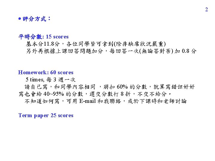
Example 2 (1) t [0, 3] (2) t [0, 3] 20

21 Fourier transform f (Hz)

22 (1) (2)

23 Example 3 left: x 1(t) = 1 for |t| 6, x 1(t) = 0 otherwise, right: x 2(t) = cos(6 t 0. 05 t 2) -axis Gabor transform t -axis

Example 4 Data source: http: //oalib. hlsresearch. com/Whales/index. html 24

25 Why Time-Frequency Analysis is Important? • Many digital signal processing applications are related to the spectrum or the bandwidth of a signal. • If the spectrum and the bandwidth can be determined adaptive, the performance can be improved. modulation, multiplexing, filter design, data compression, signal analysis, signal identification, acoustics, system modeling, radar system analysis sampling

26 Example: Generalization for sampling theory 假設有一個信號， The supporting of x(t) is t 1 t t 1 + T, x(t) 0 otherwise f The supporting of X( f ) 0 is -B f B, X( f ) 0 otherwise B 根據取樣定理， t 1/F , F =2 B, B: 頻寬 所以，取樣點數 N 的範圍是 t 1+T -B N = T/ t TF 重要定理：一個信號所需要的取樣點數的下限，等於它時頻分佈的面積 t

27 Q 1：Scaling 對於一個信號的取樣點數有沒有影響？ Hint: Q 2: How to use time-frequency analysis to reduce the number of sampling points? Time-frequency analysis is an efficient tool for adaptive signal processing.

28 時頻分析的大家族 square (1) Short-time Fourier transform (STFT) (rec-STFT, Gabor, …) (2) Wigner distribution function (WDF) improve combine improve (3) Wavelet transform (4) Time-Variant Basis Expansion spectrogram Asymmetric STFT S transform Gabor-Wigner Transform windowed WDF Cohen’s Class Distribution (Choi-Williams, Cone-Shape, Page, Levin, Kirkwood, Born-Jordan, …) Pseudo L-Wigner Distribution Haar and Daubechies Coiflet, Morlet Directional Wavelet Transform Matching Pursuit Prolate Spheroidal Wave Function (5) Hilbert-Huang Transform (唯一跳脫 Fourier transform 的架構)

29 Continuous Wavelet Transform forward wavelet transform: (t): mother wavelet, a: location, b: scaling, inverse wavelet transform: a, b(t) is dual orthogonal to (t). output Fourier transform X(f), f: frequency time-frequency analysis X(t, f), t: time, f: frequency wavelet transform X(a, b), a: time, b: scaling

30 限制： (1) when a 1 = a and b 1 = b, otherwise (2) (t) has a finite time interval Two parameters, a: 調整位置, b: 調整寬度 應用： adaptive signal analysis 思考：需要較高解析度的地方，b 的值應該如何？

31 Wavelet 的種類甚多 Mexican hat wavelet, Haar Wavelet, Daubechies wavelet, triangular wavelet, ………… 例子： Mexican hat wavelet 隨 a and b 變化之情形 a = 2, b = 1 a = 6, b = 1 a = 10, b = 1 a = 6, b = 0. 5 a = 6, b = 2 a = 6, b = 3

32 Discrete Wavelet Transform (DWT) The discrete wavelet transform is very different from the continuous wavelet transform. It is simpler and more useful than the continuous one. L-points lowpass filter g[n] N-points x[n] L-points highpass filter h[n] down sampling x. L[n] x. H[n] 2 x 1, L[n ] x[n] 的低頻成份 x 1, H[n] x[n] 的高頻成份 down sampling 2

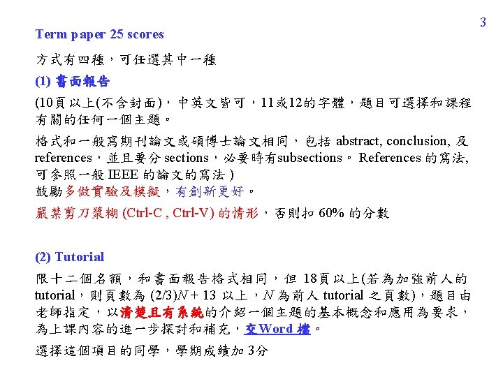
33 例子： 2 -point Haar wavelet g[n] = 1/2 for n = − 1, 0 g[n] = 0 otherwise g[n] ½ ½ -3 -2 -1 0 1 2 3 n then (兩點平均) h[0] = 1/2, h[− 1] = − 1/2, h[n] = 0 otherwise h[n] ½ -3 -2 -1 0 1 2 3 n -½ (兩點之差)

34 Discrete wavelet transform 有很多種 (discrete Haar wavelet, discrete Daubechies wavelet, B-spline DWT, symlet, coilet, ……. . ) 一般的 wavelet, g[n] 和 h[n] 點數會多於 2 點 但是 g[n] 通常都是 lowpass filter 的型態 h[n] 通常都是 highpass filter 的型態

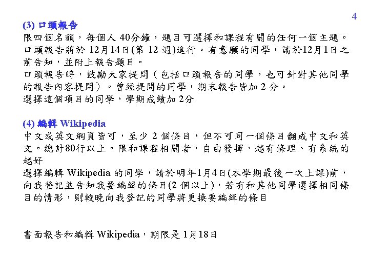
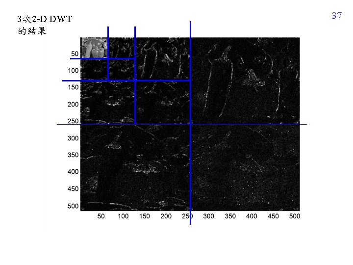
35 2 -D 的情形 L-points M ×N x[m, n] g[n] 2 along n L-points h[n] 2 along n n m v 1, L[m, n] x[m, n] v 1, H[m, n] g[m] 2 along m x 1, L[m, n] m 低頻, n 低頻 h[m] 2 along m x 1, H 1[m, n] m 高頻, n 低頻 g[m] 2 along m x 1, H 2[m, n] m 低頻, n 高頻 2 h[m] along m x 1, H 3[m, n] m 高頻, n 高頻

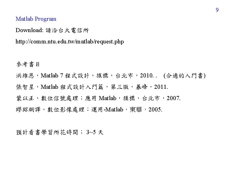
36 原影像 Pepper. bmp x 1, L[m, n] x 1, H 2[m, n] 2 -D DWT 的結果 x 1, H 1[m, n] x 1, H 3[m, n]

38 應用： 影像壓縮 (JPEG 2000) 其他應用：edge detection corner detection filter design pattern recognition music signal processing economical data temperature analysis feature extraction biomedical signal processing

有些聲音檔是 雙聲道 （Stereo）的型態 (俗稱立體聲) 例： [x, fs]=wavread('C: WINDOWSMedianotify. wav'); size(x) = 29823 2 fs = 22050 42

43 B. 繪出頻譜 X = fft(x); abs(X)*dt plot(abs(X)*dt); % dt = 1/fs ringin. wav 的頻譜 m fft 橫軸 轉換的方法 (1) Using normalized frequency F: F = m / N. (2) Using frequency f, f = F fs = m (fs / N).

44 abs(X)*dt ringin. wav 的頻譜 F abs(X)*dt ringin. wav 的頻譜 f

E. 用 Matlab 錄音的方法 錄音之前，要先將電腦接上麥克風，且確定電腦有音效卡 (部分的 notebooks 不需裝麥克風即可錄音) 範例程式： Sec = 3; Fs = 8000; recorder = audiorecorder(Fs, 16, 1); recordblocking(recorder, Sec); audioarray = getaudiodata(recorder); 執行以上的程式，即可錄音。 錄音的時間為三秒，sampling frequency 為 8000 Hz 錄音結果為 audioarray，是一個 column vector (如果是雙聲道，則是 兩個 column vectors) 47

範例程式 (續)： wavplay(audioarray, Fs); % 播放錄音的結果 t = [0: length(audioarray)-1]. /Fs; plot (t, audioarray‘); % 將錄音的結果用圖畫出來 xlabel('sec', 'Font. Size', 16); wavwrite(audioarray, Fs, ‘test. wav’) % 將錄音的結果存成 *. wav 檔 48

49 指令說明： recorder = audiorecorder(Fs, nb, nch); Fs: sampling frequency, (提供錄音相關的參數) nb: using nb bits to record each data nch: number of channels (1 or 2) recordblocking(recorder, Sec); (錄音的指令) recorder: the parameters obtained by the command “audiorecorder” Sec: the time length for recording audioarray = getaudiodata(recorder); (將錄音的結果，變成 audioarray 這個 column vector，如果是 雙聲道，則 audioarray 是兩個 column vectors) 以上這三個指令，要並用，才可以錄音

50 F、MP 3 檔的讀和寫 要先去這個網站下載 mp 3 read. m, mp 3 write. m 的程式 http: //www. mathworks. com/matlabcentral/fileexchange/13852 -mp 3 readand-mp 3 write 程式原作者：Dan Ellis mp 3 read. m : 讀取 mp 3 的檔案 mp 3 write. m : 製作 mp 3 的檔案 不同於 *. wav 檔 (未壓縮過的聲音檔)，*. mp 3 是經過 MPEG-2 Audio Layer III的技術壓縮過的聲音檔

51 範例： %% Write an MP 3 file by Matlab fs=8000; % sampling frequency t = [1: fs*3]/3; filename = ‘test’; Nbit=32; % number of bits per sample x= 0. 2*cos(2*pi*(500*t+300*(t-1. 5). ^3)); mp 3 write(x, fs, Nbit, filename); % make an MP 3 file test. mp 3 %% Read an MP 3 file by Matlab [x 1, fs 1]=mp 3 read('phase 33. mp 3'); x 2=x 1(577: end); % delete the head sound(x 2, fs 1)