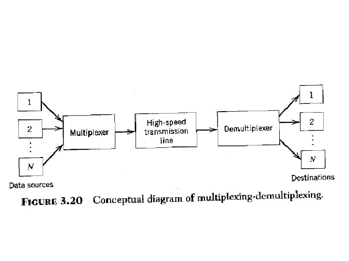
Time Division Multiplexing allows multiple devices to communicate


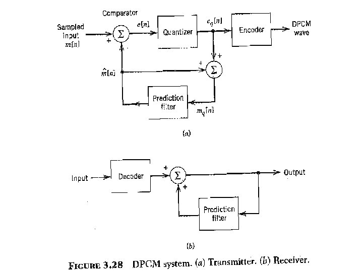
![Differential Pulse Code Modulation(DPCM) transmitter m[n] – unquantized input sample m^[n] – predicted value](https://slidetodoc.com/presentation_image_h2/aec5278d13b3033cb28fb73427a9d4eb/image-28.jpg "Differential Pulse Code Modulation(DPCM) transmitter m[n] – unquantized input sample m^[n] – predicted value")
 transmitter")
 q. Differential Pulse Code Modulation (DPCM) is a procedure")
 q. It often happens that in the analogical signals,")
 Can save bandwidth by not sending all samples. *")


 Receiver")


 – A single-bit PCM code to achieve digital transmission of analog.")


 • To increase")

 can't")

- Slides: 59
Time Division Multiplexing allows multiple devices to communicate over the same circuit by assigning time slots for each device on the line.
Parameter Working No. of Slots Buffers Synchronous TDM In Synchronous TDM data flow of each input connection is divided into units and each input occupies one output time slot. In Synchronous TDM no. of slots in each frame are equal to no. of input lines. Buffering is not done, frame is sent after a particular interval of time whether someone has data to send or not. Statistical TDM In Statistical TDM slots are allotted dynamically. i. e. input line is given slots in output frame if and only if it has data to send. In Statistical TDM, No. of slots in each frame are less than the no. of input lines. Buffering is done and only those inputs are given slots in output frame whose buffer contains data to send.
Addressing Slots in Synchronous TDM carry data only and there is no need of addressing. Synchronization and pre assigned relationships between input and outputs that serve as an address. Synchronization bits are on used at the beginning of each frame. Capacity Max. Bandwidth utilization if all inputs have data to send. Slots in Statistical TDM contain both data and address of the destination. No synchronization bits are used The capacity of link is normally is less than the sum of the capacity of each channel.
1 2 3 4 T 1 6. 312 Mb/s 2 7 T 2 system – combination of 4 T 1 system T 3 system – combination of 7 T 2 system T 4 system – combination of 6 T 3 system 44. 736 Mb/s 1 2 6 T 3 Fourth level multiplexer S 24 1. 544 Mb/s Third level multiplexer S 2 T 1 CARRIER SYSTEM Accommodate 24 voice channels each frame 24 words -125µs – 1 sync bi each word - 8 -bits sampling rate – 8 KHz duration of each bit= 0. 647 µs transmission rate 1. 544 Mbps T 2 1 Second level multiplexer S 1 First level multiplexer TDM HIERARCHY 274. 176 Mb/s T 4
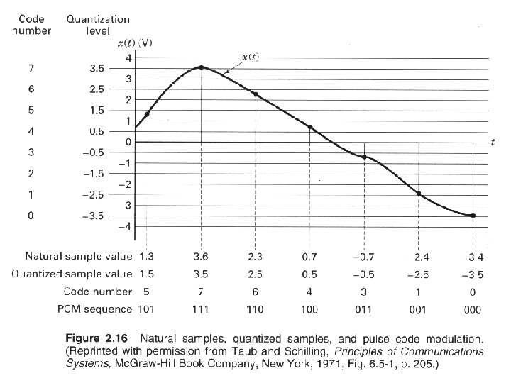
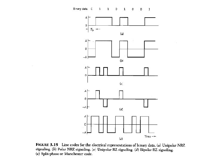
Bandwidth-Noise Tradeoff • Continuous wave modulation like FM and analog pulse modulation like PPM have Figure of merit propotional to square of transmission bandwidth. • Digital pulse modulation like PCM provides better tradeoff than square law. • In PCM , sampling does discrete time representation of message signal and quantization does discrete amplitude representation of message signal. • By representing message signal as coded binary pulses PCM provides better trade off between bandwidth and noise.
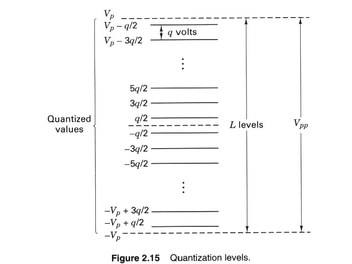
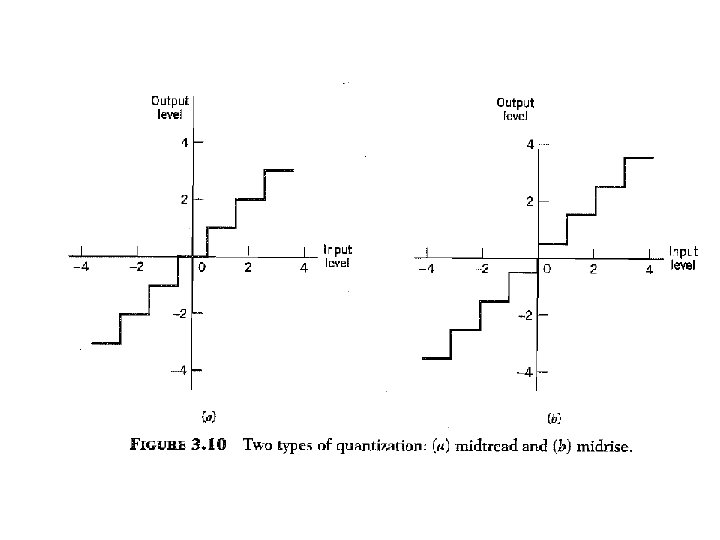
Quantization
In non uniform quantization the step size increase as the separation from origin increase. Weak passage voice signals which occur frequently are favored than rarely occuring voice signals with high amplitude.
Non uniform quantization is equivalent to applying compressed base band signal to uniform quantizer
DERIVATION-SNR OF UNIFORM QUANTIZER
DERIVATION-SNR OF UNIFORM QUANTIZER
DERIVATION-SNR OF UNIFORM QUANTIZER
DERIVATION-SNR OF UNIFORM QUANTIZER
Quantization
Quantization
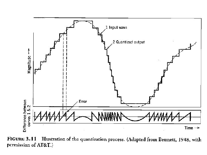
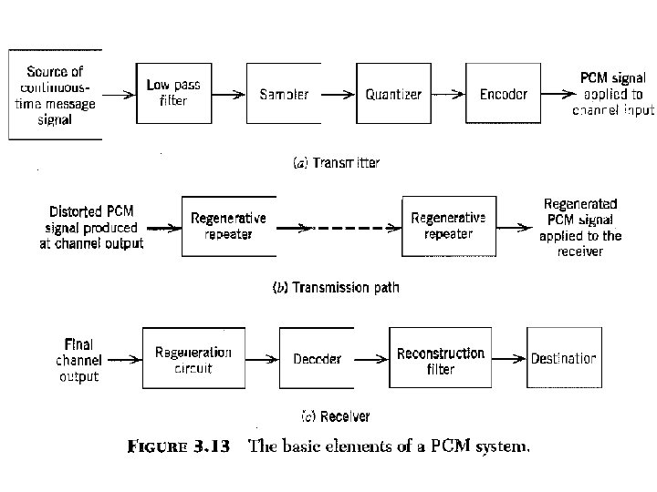
Regenerative repeaters are present at sufficiently close spacing along the transmission route to control the effect of distortion and noise
Error Threshold
VIRTUES, LIMITATIONS & MODIFICATIONS OF PCM
Differential Pulse Code Modulation(DPCM) transmitter m[n] – unquantized input sample m^[n] – predicted value e[n] – prediction error (or) difference between unquantized input sample and prediction of it q[n] – quantization error mq[n] – prediction filter output
Differential Pulse Code Modulation(DPCM) transmitter
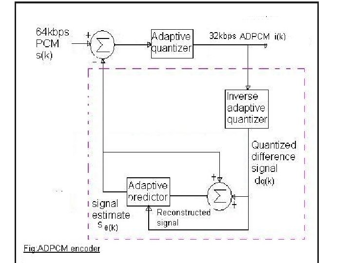
Differential Pulse Code Modulation (DPCM) q. Differential Pulse Code Modulation (DPCM) is a procedure of converting an analog into a digital signal in which an analog signal is sampled and then the difference between the actual sample value and its predicted value (predicted value is based on previous sample or samples) is quantized and then encoded forming a digital value. q. DPCM code words represent differences between samples unlike PCM where code words represented a sample value. EKT 343 -Principles of Communication Engineering 30
Differential Pulse Code Modulation (DPCM) q. It often happens that in the analogical signals, which are coded in PCM (voices, images, etc), that many next samples show the same quantization level; as a consequence there is the transmission of many equal PCM codes and this is redundant for the reception signal reconstruction. q. The DPCM coding exploits this redundancy between adjacent samples. q. DPCM requires fewer bits than the standard PCM. EKT 343 -Principles of Communication Engineering 31
Differential Pulse Code Modulation (DPCM) Can save bandwidth by not sending all samples. * Send true samples occasionally. * In between, send only change from previous value. * Change values can be sent using a fewer number of bits than true samples. Examples (CCITT standards) * 32 k bits / s (4 -bit quantization and 8 k samples /s) for 3. 2 k. Hz * 64 k bits / s (4 -bit quantization and 16 k samples /s) for 7 k. Hz
How it works – the background • We know the signal up to a certain time • Use prediction to estimate future values • Signal sampled at fs= 1/Ts ; sampled sequence – {m[n]}, where samples are Ts seconds apart • Input signal to the quantizer – difference between the unquantized input signal m(t) and its prediction: prediction of the input sample Digital Communication Systems 2012 R. Sokullu 33/45
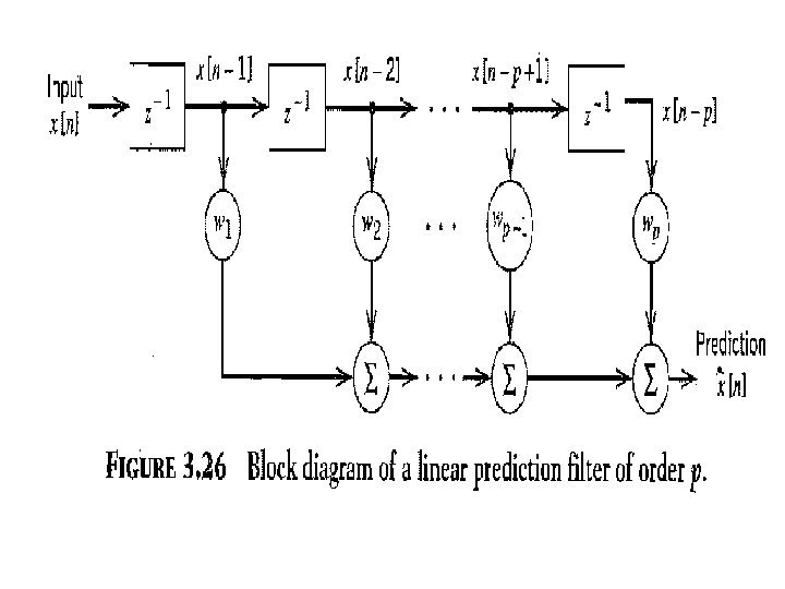
• Predicted value – achieved by linear prediction filter whose input is the quantized version of the input sample m[n]. • The difference e[n] is the prediction error (what we expect and what actually happens) • By encoding the quantizer output we actually create a variation of PCM called differential PCM (DPCM). Digital Communication Systems 2012 R. Sokullu 34/45
Receiver side • decoder – constructs the quantized error signal • quantized version of the input is recovered by using the same prediction filter as at the tx • if there is no channel noise – encoded input to the decoder is identical to the transmitter output • then the receiver output will be equal to mq[n] (differs from m[n] by q[n] caused by quantizing the prediction error e[n]) Digital Communication Systems 2012 R. Sokullu 35/45
Differential Pulse Code Modulation(DPCM) Receiver
PROCESSING GAIN
PROCESSING GAIN
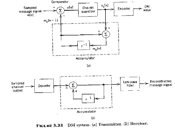
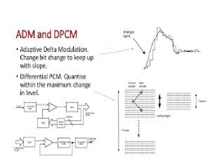
Delta Modulation
Delta Modulation (DM) – A single-bit PCM code to achieve digital transmission of analog. Use only 1 bit either logic ‘ 1’ or ‘ 0’. – Logic ‘ 0’ is transmitted if current sample is smaller than the previous sample – Logic ‘ 1’ is transmitted if current sample is larger than the previous sample EKT 343 -Principles of Communication Engineering 43
Cont’d… EKT 343 -Principles of Communication Engineering 44
DELTA MODULATION SYSTEM
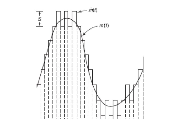
Cont’d. . . • Analog input is approximated by a staircase function • Move up or down one level ( ) at each sample interval (by one quantization level at each sampling time) output of DM is a single bit. • Binary behavior – Function moves up or down at each sample interval • In DM the quantization levels are represented by two symbols: 0 for - and 1 for +. In fact the coding process is performed on eq. • The main advantage of DM is its simplicity. EKT 343 -Principles of Communication Engineering 47
Delta Modulation - Example EKT 343 -Principles of Communication Engineering 48
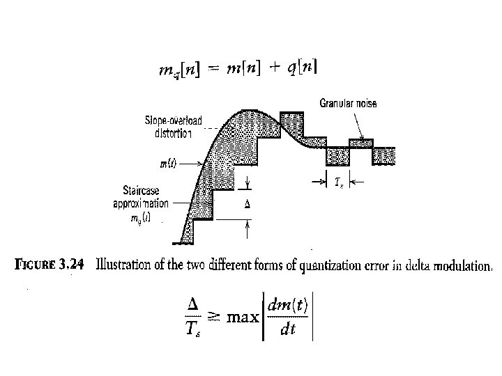
Noise in Delta Modulation Systems • slope overhead distortion • granular noise Digital Communication Systems 2012 R. Sokullu 51/45
Slope Overhead Distortion • The quantized message signal can be represented as: • where the input to the quantizer can be represented as: Sample of m(T) at time n. T Quantizer input at time (n -1)T So, (except for the quantization error) the quantizer input is the first backward difference (derivative) of the input signal = inverse of the digital integration process Digital Communication Systems 2012 R. Sokullu 52/45
Discussion • Consider the max slope of the input signal m(t) • To increase the samples {mq[n]} as fast as the input signal in its max slope region the following condition should be fulfilled: otherwise the step-size Δ is too small Digital Communication Systems 2012 R. Sokullu 53/45
Granular Noise • • In contrast to slope overhead Occurs when step size is too large Usually relatively flat segment of the signal Analogous to quantization noise in PCM systems Digital Communication Systems 2012 R. Sokullu 54/45
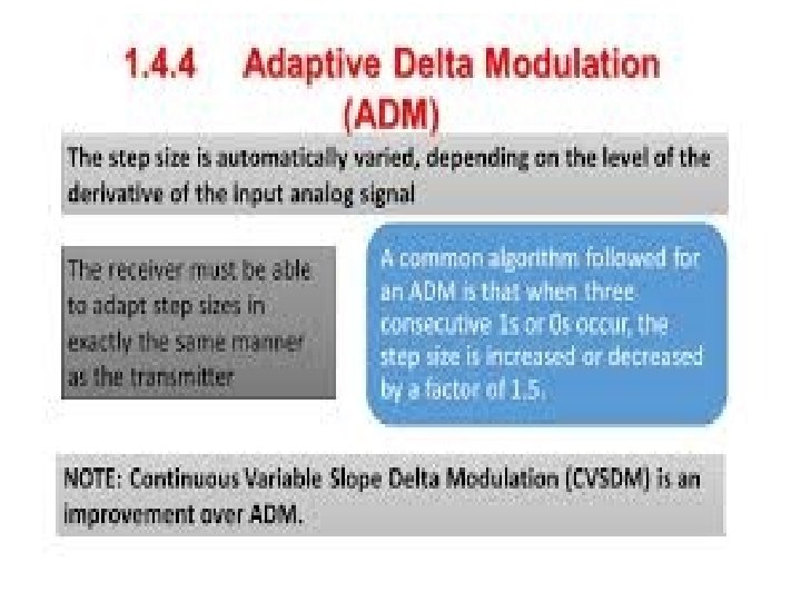
q Slope overload distortion occurs when is too small, the staircase approximation mq(t) can't follow closely the actual curve of the message signal m(t ). q large is needed for rapid variations of m(t) to reduce the slope-overload distortion q granular noise occurs when is too large relative to the local slope characteristics of m(t). q granular noise is similar to quantization noise in PCM q small is needed for slowly varying m(t) to reduce the granular noise EKT 343 -Principles of Communication Engineering 55
Comparison • DPCM and DM – DPCM includes DM as a special case – Similarities • subject to slope-overhead and quantization error – Differences • DM uses a 1 -bit quantizer • DM uses a single delay element (zero prediction order) • DPCM and PCM – both DM and DPCM use feedback while PCM does not – all subject to quantization error Digital Communication Systems 2012 R. Sokullu 59/45