Tide Simulation Using Regional Ocean Modeling System ROMS

Tide Simulation Using Regional Ocean Modeling System (ROMS) Xiaochun Wang Co-author: Changming Dong, Yi Chao, Zhijin Li, James Mc. Willams Contributions from: Koji Matsumoto, John Farrara, Jei-kook Choi, Quoc Vu ROMS/TOMS Workshop Oct. 24 -26 2005

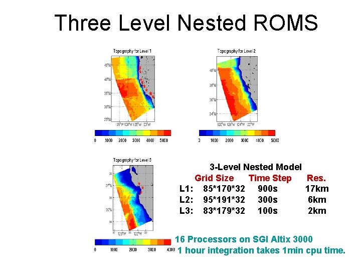
Three Level Nested ROMS 3 -Level Nested Model Grid Size Time Step L 1: 85*170*32 900 s L 2: 95*191*32 300 s L 3: 83*179*32 100 s Res. 17 km 6 km 2 km 16 Processors on SGI Altix 3000 1 hour integration takes 1 min cpu time.

Boundary Conditions • Open Boundary Condition SSH: Chapman condition Tangential Barotropic Velocity: Oblique radiation Normal Barotropic Velocity: Flather condition • Closed Boundary Condition SSH: Zero gradient Tangential Velocity: Free slip Normal Velocity: Zero Tide SSH and transport are from the barotropic tide data assimilation system of Oregon State University (TPXO. 6). Atmospheric Forcing: Hourly wind stress and heat flux.

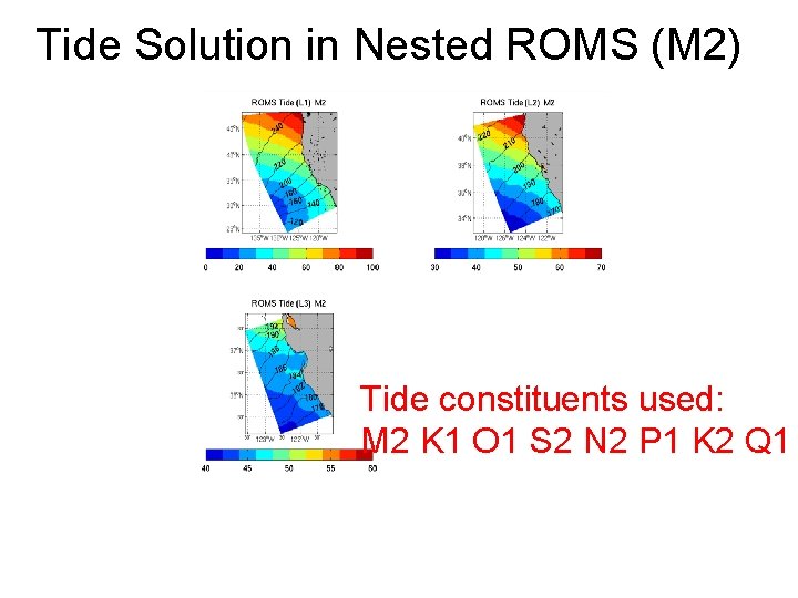
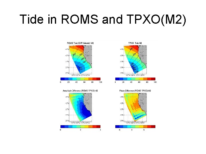
Tide Solution in Nested ROMS (M 2) Tide constituents used: M 2 K 1 O 1 S 2 N 2 P 1 K 2 Q 1

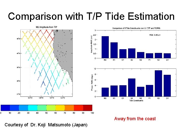
Comparison with T/P Tide Estimation Away from the coast Courtesy of Dr. Koji Matsumoto (Japan)

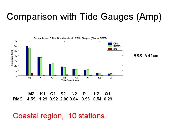
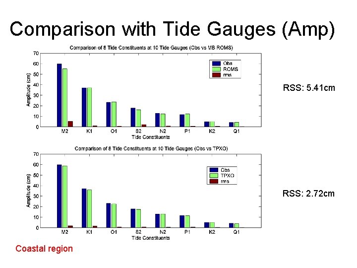
Comparison with Tide Gauges (Amp) RSS: 5. 41 cm RMS M 2 K 1 O 1 S 2 N 2 P 1 K 2 Q 1 4. 59 1. 29 0. 92 2. 00 0. 64 0. 93 0. 54 0. 29 Coastal region, 10 stations.

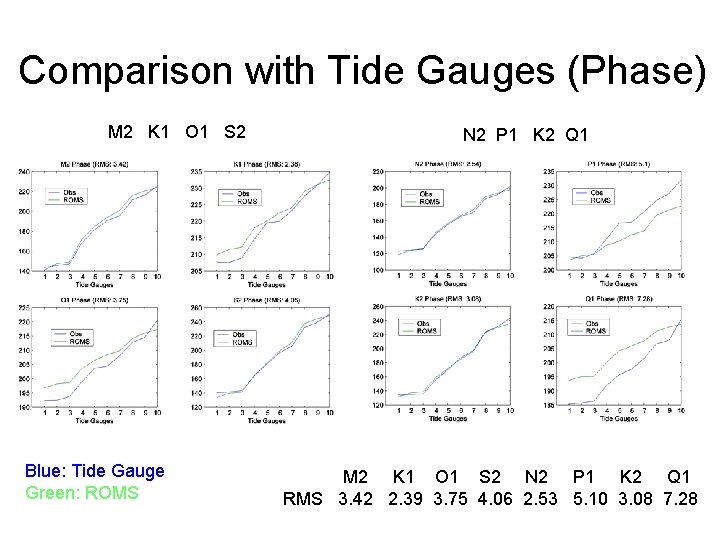
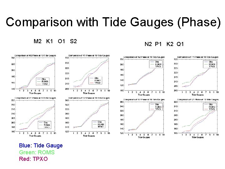
Comparison with Tide Gauges (Phase) M 2 K 1 O 1 S 2 Blue: Tide Gauge Green: ROMS N 2 P 1 K 2 Q 1 M 2 K 1 O 1 S 2 N 2 P 1 K 2 Q 1 RMS 3. 42 2. 39 3. 75 4. 06 2. 53 5. 10 3. 08 7. 28

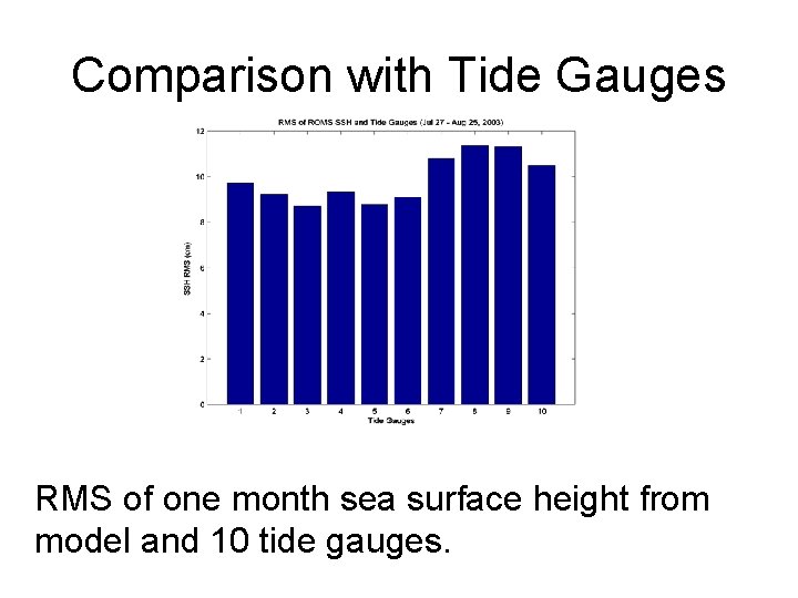
Comparison with Tide Gauges RMS of one month sea surface height from model and 10 tide gauges.

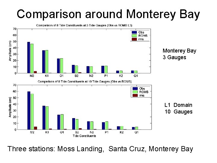
Comparison around Monterey Bay 3 Gauges L 1 Domain 10 Gauges Three stations: Moss Landing, Santa Cruz, Monterey Bay

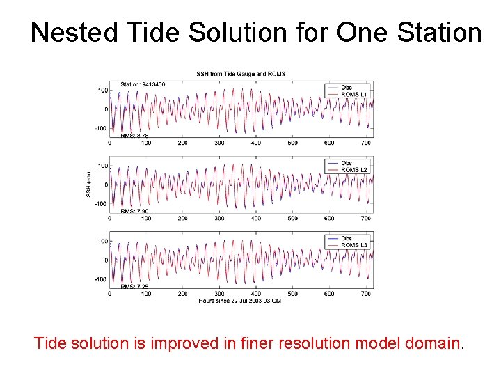
Nested Tide Solution for One Station Tide solution is improved in finer resolution model domain.

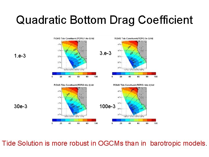
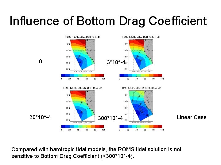
Quadratic Bottom Drag Coefficient 1. e-3 30 e-3 100 e-3 Tide Solution is more robust in OGCMs than in barotropic models.

Future Plan • Tidal Data Assimilation Find optimal boundary condition • Tidal Current Simulation How to improve the tide current

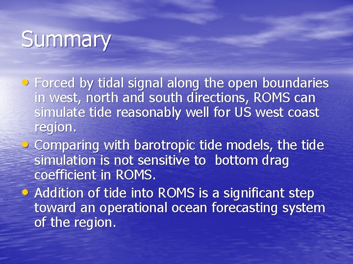
Summary • Forced by tidal signal along the open boundaries • • in west, north and south directions, ROMS can simulate tide reasonably well for US west coast region. Comparing with barotropic tide models, the tide simulation is not sensitive to bottom drag coefficient in ROMS. Addition of tide into ROMS is a significant step toward an operational ocean forecasting system of the region.

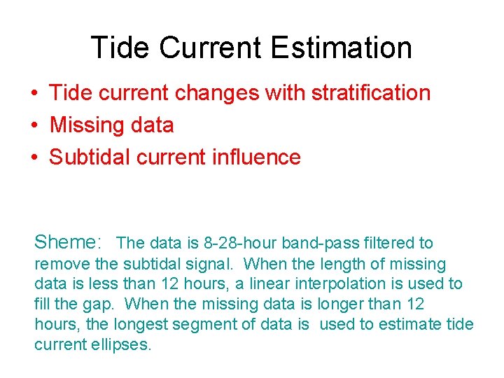
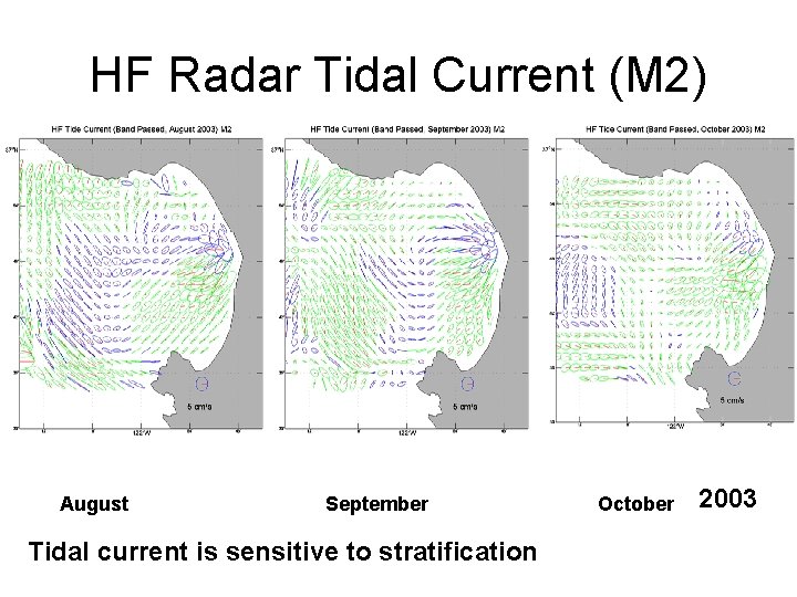
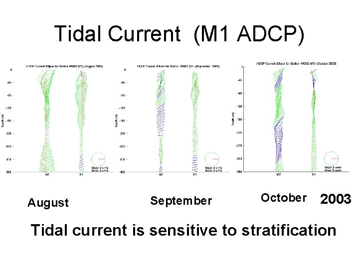
Tide Current Estimation • Tide current changes with stratification • Missing data • Subtidal current influence Sheme: The data is 8 -28 -hour band-pass filtered to remove the subtidal signal. When the length of missing data is less than 12 hours, a linear interpolation is used to fill the gap. When the missing data is longer than 12 hours, the longest segment of data is used to estimate tide current ellipses.

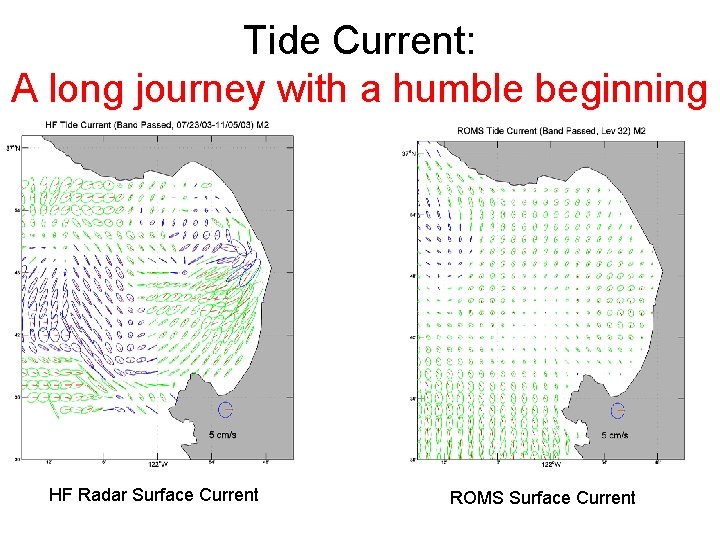
Tide Current: A long journey with a humble beginning HF Radar Surface Current ROMS Surface Current

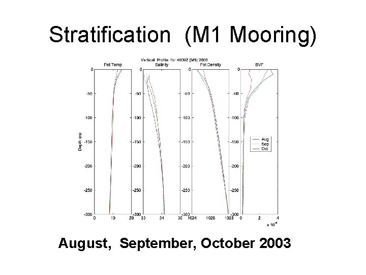
Stratification (M 1 Mooring) August, September, October 2003

HF Radar Tidal Current (M 2) August September Tidal current is sensitive to stratification October 2003

Tidal Current (M 1 ADCP) August September October 2003 Tidal current is sensitive to stratification

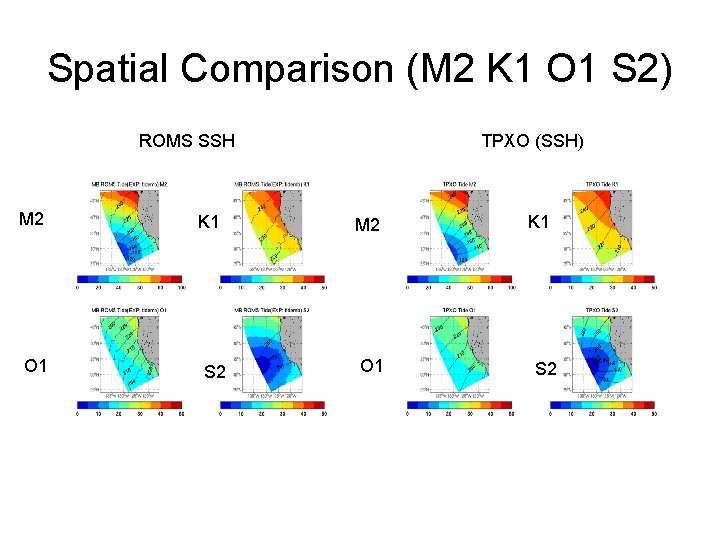
Spatial Comparison (M 2 K 1 O 1 S 2) ROMS SSH M 2 O 1 K 1 S 2 TPXO (SSH) M 2 O 1 K 1 S 2

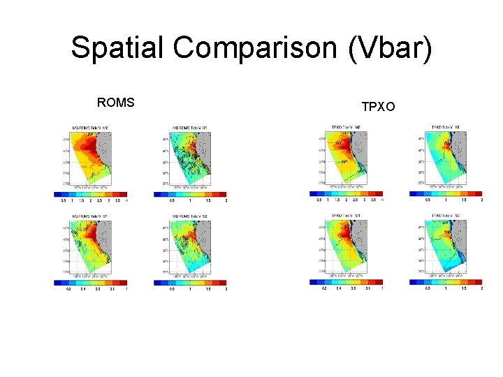
Spatial Comparison (Vbar) ROMS TPXO

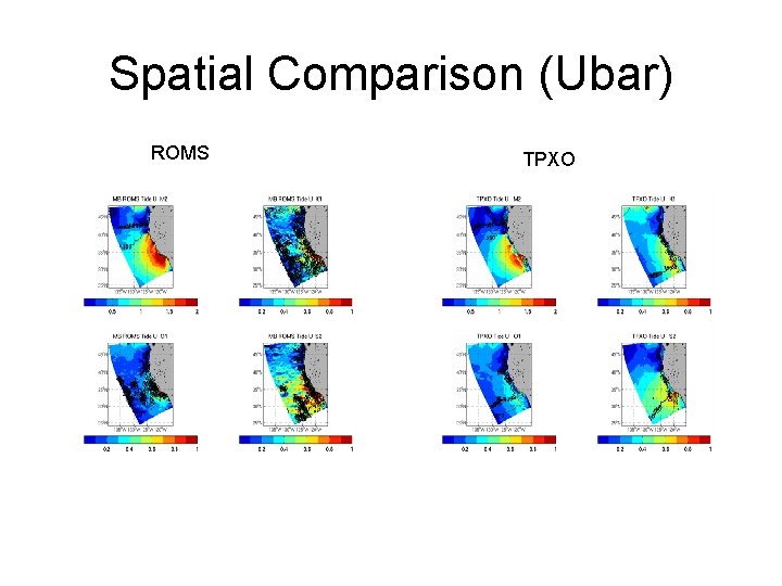
Spatial Comparison (Ubar) ROMS TPXO

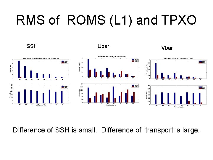
RMS of ROMS (L 1) and TPXO SSH Ubar Vbar Difference of SSH is small. Difference of transport is large.

Influence of Bottom Drag Coefficient 0 30*10^-4 300*10^-4 Linear Case Compared with barotropic tidal models, the ROMS tidal solution is not sensitive to Bottom Drag Coefficient (<300*10^-4).

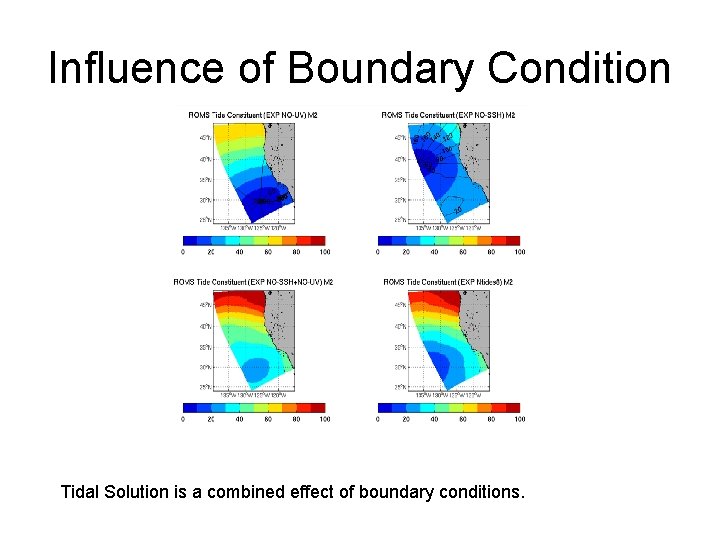
Influence of Boundary Condition Tidal Solution is a combined effect of boundary conditions.

Tide in ROMS and TPXO(M 2)

Comparison with Tide Gauges (Amp) RSS: 5. 41 cm RSS: 2. 72 cm Coastal region

Comparison with Tide Gauges (Phase) M 2 K 1 O 1 S 2 Blue: Tide Gauge Green: ROMS Red: TPXO N 2 P 1 K 2 Q 1