Thursday 19 February Lecture 14 Classification Reading Estimating

Thursday 19 February Lecture 14: Classification Reading: “Estimating Sub-pixel Surface Roughness Using Remotely Sensed Stereoscopic Data” pdf preprint for RSE available on class website Last lecture: Spectral Mixture Analysis

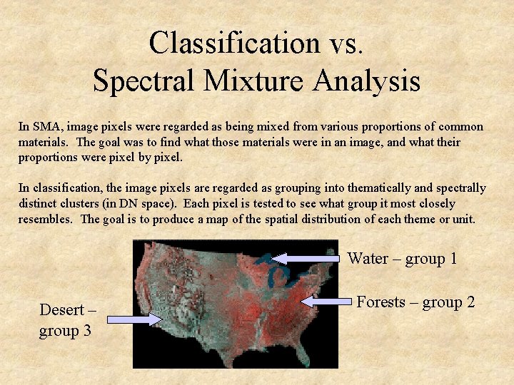
Classification vs. Spectral Mixture Analysis In SMA, image pixels were regarded as being mixed from various proportions of common materials. The goal was to find what those materials were in an image, and what their proportions were pixel by pixel. In classification, the image pixels are regarded as grouping into thematically and spectrally distinct clusters (in DN space). Each pixel is tested to see what group it most closely resembles. The goal is to produce a map of the spatial distribution of each theme or unit. Water – group 1 Desert – group 3 Forests – group 2

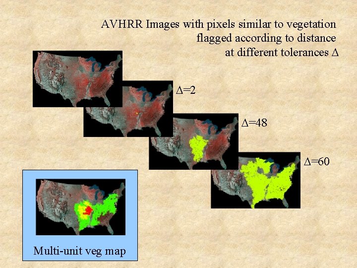
AVHRR Images with pixels similar to vegetation flagged according to distance at different tolerances D D=2 D=48 D=60 Multi-unit veg map

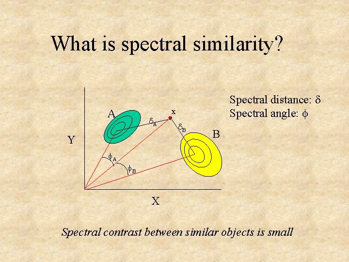
What is spectral similarity? A d. A Y A Spectral distance: d Spectral angle: x d. B B B X Spectral contrast between similar objects is small

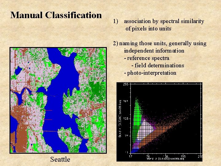
Manual Classification 1) association by spectral similarity of pixels into units 2) naming those units, generally using independent information - reference spectra - field determinations - photo-interpretation Seattle

Basic steps in image classification: 1) Data reconnaissance and self-organization 2) Application of the classification algorithm 3) Validation

Reconnaissance and data organization Reconnaissance What is in the scene? What is in the image? What bands are available? What questions are you asking of the image? Can they be answered with image data? Are the data sufficient to distinguish what’s in the scene? Organization of data How many data clusters in n-space can be recognized? What is the nature of the cluster borders? Do the clusters correspond to desired map units?

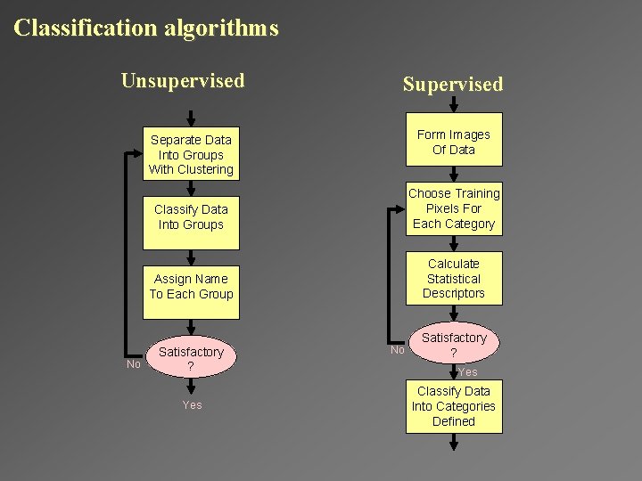
Classification algorithms Unsupervised Supervised Form Images Of Data Separate Data Into Groups With Clustering No Classify Data Into Groups Choose Training Pixels For Each Category Assign Name To Each Group Calculate Statistical Descriptors Satisfactory ? Yes No Satisfactory ? Yes Classify Data Into Categories Defined

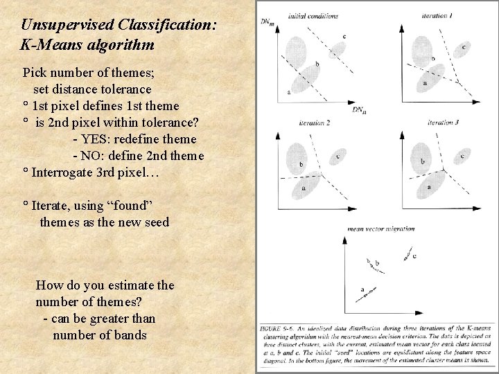
Unsupervised Classification: K-Means algorithm Pick number of themes; set distance tolerance ° 1 st pixel defines 1 st theme ° is 2 nd pixel within tolerance? - YES: redefine theme - NO: define 2 nd theme ° Interrogate 3 rd pixel… ° Iterate, using “found” themes as the new seed How do you estimate the number of themes? - can be greater than number of bands

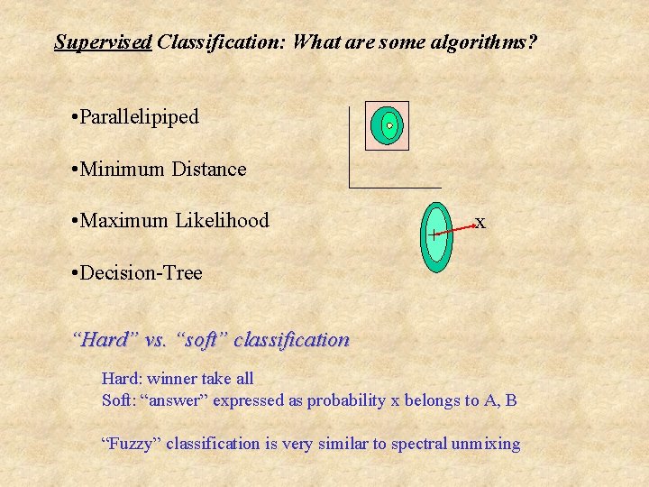
Supervised Classification: What are some algorithms? • Parallelipiped • Minimum Distance • Maximum Likelihood + x • Decision-Tree “Hard” vs. “soft” classification Hard: winner take all Soft: “answer” expressed as probability x belongs to A, B “Fuzzy” classification is very similar to spectral unmixing

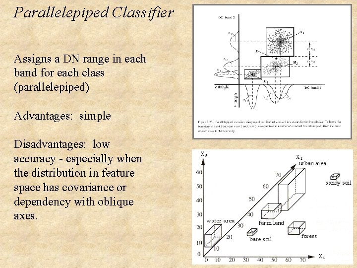
Parallelepiped Classifier Assigns a DN range in each band for each class (parallelepiped) Advantages: simple Disadvantages: low accuracy - especially when the distribution in feature space has covariance or dependency with oblique axes.

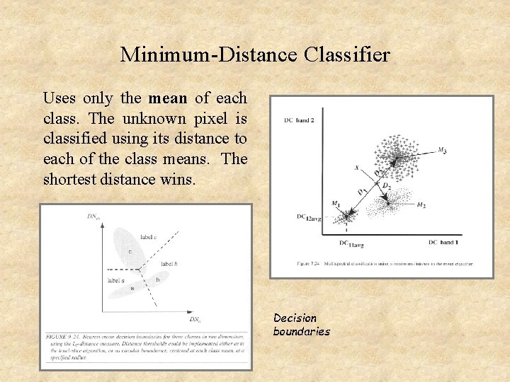
Minimum-Distance Classifier Uses only the mean of each class. The unknown pixel is classified using its distance to each of the class means. The shortest distance wins. Decision boundaries

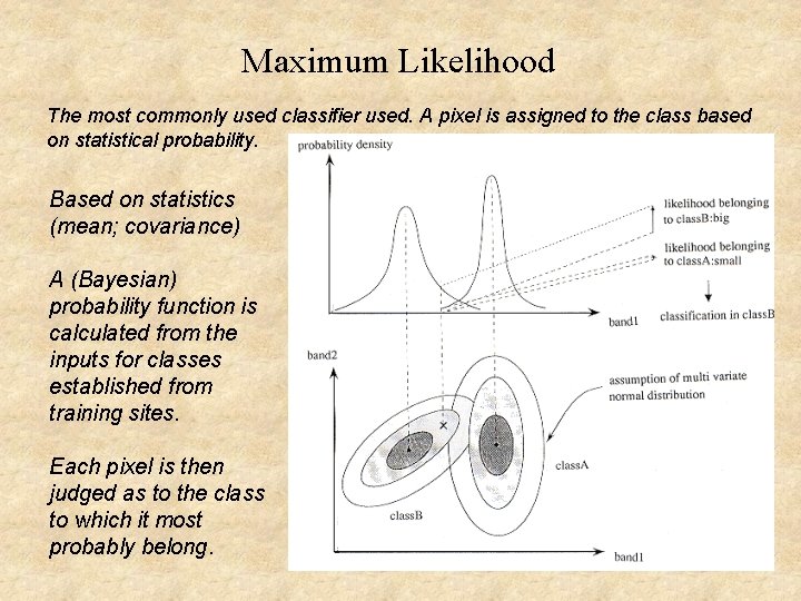
Maximum Likelihood The most commonly used classifier used. A pixel is assigned to the class based on statistical probability. Based on statistics (mean; covariance) A (Bayesian) probability function is calculated from the inputs for classes established from training sites. Each pixel is then judged as to the class to which it most probably belong.

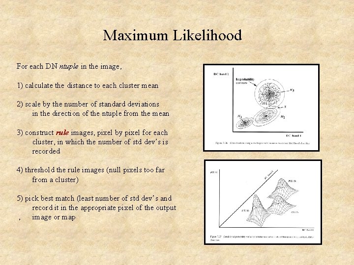
Maximum Likelihood For each DN ntuple in the image, 1) calculate the distance to each cluster mean 2) scale by the number of standard deviations in the direction of the ntuple from the mean 3) construct rule images, pixel by pixel for each cluster, in which the number of std dev’s is recorded 4) threshold the rule images (null pixels too far from a cluster) 5) pick best match (least number of std dev’s and record it in the appropriate pixel of the output , image or map

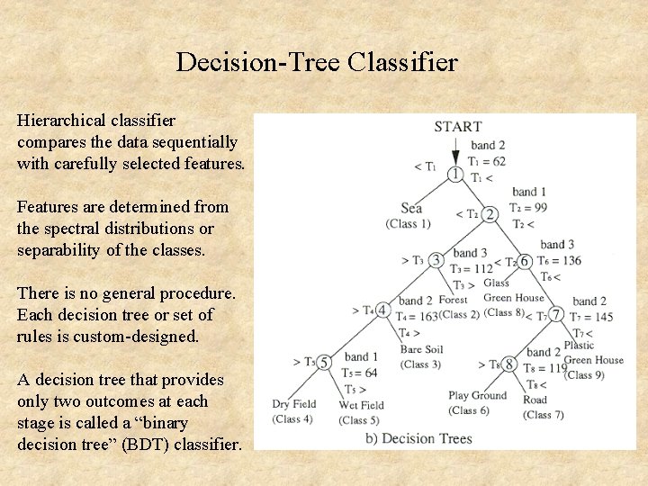
Decision-Tree Classifier Hierarchical classifier compares the data sequentially with carefully selected features. Features are determined from the spectral distributions or separability of the classes. There is no general procedure. Each decision tree or set of rules is custom-designed. A decision tree that provides only two outcomes at each stage is called a “binary decision tree” (BDT) classifier.

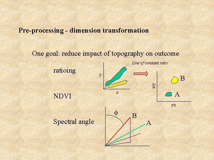
Pre-processing - dimension transformation One goal: reduce impact of topography on outcome Line of constant ratio y B x/y ratioing NDVI A x y/z Spectral angle B A

Validation Photointerpretation Look at the original data: does your map make sense to you?

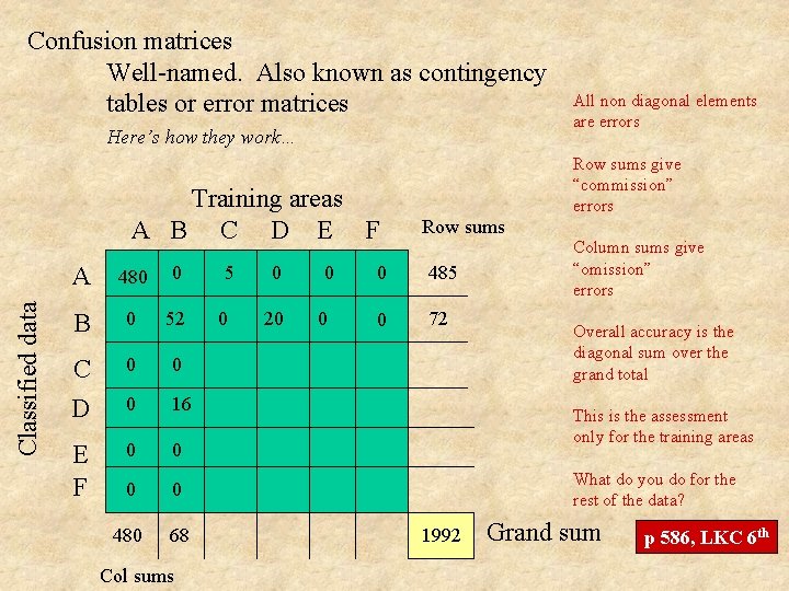
Confusion matrices Well-named. Also known as contingency tables or error matrices Here’s how they work… Classified data Training areas A B C D E F A 480 0 B 0 52 C D 0 0 0 16 E F 0 0 480 68 Col sums 5 0 0 20 0 0 All non diagonal elements are errors Row sums give “commission” errors Row sums 0 485 0 72 Column sums give “omission” errors Overall accuracy is the diagonal sum over the grand total This is the assessment only for the training areas What do you do for the rest of the data? 1992 Grand sum p 586, LKC 6 th

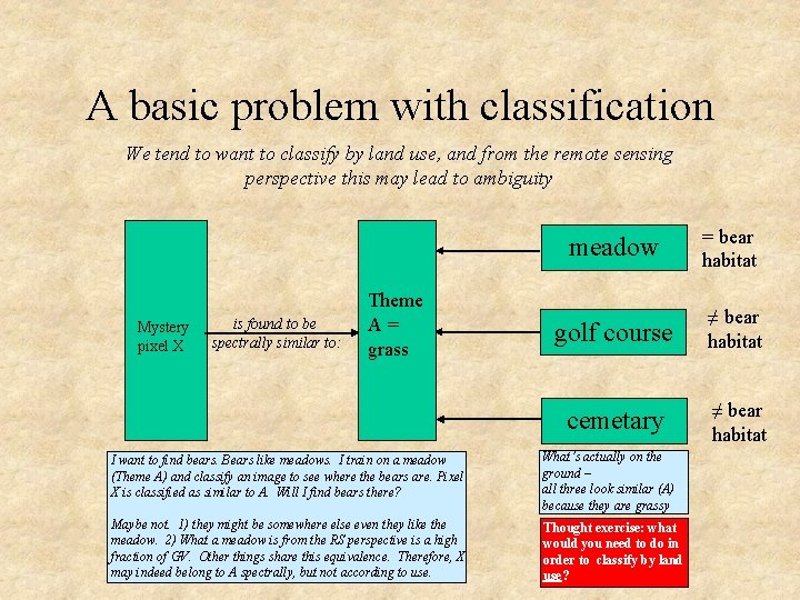
A basic problem with classification We tend to want to classify by land use, and from the remote sensing perspective this may lead to ambiguity Mystery pixel X is found to be spectrally similar to: Theme A= grass meadow = bear habitat golf course ≠ bear habitat cemetary ≠ bear habitat I want to find bears. Bears like meadows. I train on a meadow (Theme A) and classify an image to see where the bears are. Pixel X is classified as similar to A. Will I find bears there? What’s actually on the ground – all three look similar (A) because they are grassy Maybe not. 1) they might be somewhere else even they like the meadow. 2) What a meadow is from the RS perspective is a high fraction of GV. Other things share this equivalence. Therefore, X may indeed belong to A spectrally, but not according to use. Thought exercise: what would you need to do in order to classify by land use?

Next class: Relative dating of surfaces on Mars – counting craters (Matt Smith, ESS)