Thunderstorm In Situ Measurements from the Armored T

Thunderstorm In Situ Measurements from the Armored T 28 Aircraft: Classification of 2 D Probe Hydrometeor Images Rand Feind

Overview • • • The problem The data Classes Feature Selection Classifiers Results

The Problem • Sensor on T-28 collects images • Number of images can number in the hundreds of thousands • Hydrometeor classification provides key to estimating cloud characteristics

2 DC and HVPS Probes

The Data • Strips taken from the sensor • Treated as black/white images • 2000 images extracted for training and testing

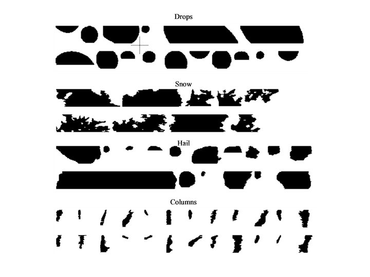
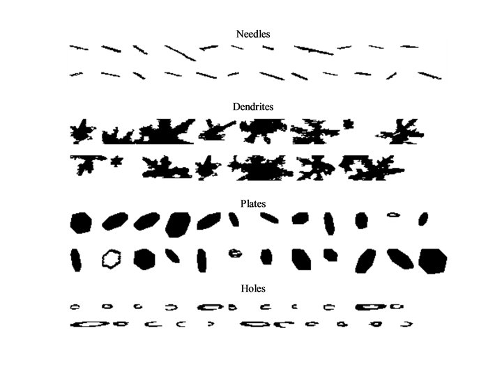
The Classes 1. Drops - smooth perimeters; appear to be circular 2. Snow - irregular, convoluted perimeters 3. Hail - somewhat rough, lumpy perimeters; appear to be circular 4. Columns - linear like needles but wider; can have rough perimeters 5. Needles - linear and narrow 6. Dendrites - like snow but evidence of 6 -way symmetry 7. Plates - appear to be planar and 6 -sided 8. Holes - anomalous images (due to probe tip shedding)

Feature Selection • Need to select features for classification • How many? – Literature search for ideas – Start with many, eliminate (started with 25) • Elimination using divergence measure – Provided base set of 6 • Trial and error – Add one at a time, check error – Delete one of 6, check error

Example : Basic Metrics • X Dimension - The width of the image in pixels along the flight direction (xdimension) (e. g. , the horizontal dimension). • Y Dimension - The height of the image in pixels perpendicular to the flight direction (y-dimension) (e. g. , the vertical dimension). Note: In the case of the T-28, this orientation is perpendicular to the wingspan. • Heymsfield Diameter - The larger of the X Dimension and the Y Dimension above.

Basic Metrics • Bottom Occulted - If the 32 photodetectors in the 2 DC probe are numbered 1 through 32, this metric is the number of times photodetector 1 is shaded (i. e. , the number of image pixels along the bottom edge of the image window). • Top Occulted - Same as Bottom Occulted except photodetector 32 or the top edge of the image window. • Total Occulted – Sum of the previous two features. Used as a particle rejection criterion in Holroyd, 1987.

Basic Metrics • Pixel Area – Sum of the number of pixels comprising a 2 D image. • Area – Area of the particle image in square micrometers (um). • Streak – Ratio of the x-dimension to the y-dimension. Used to detect anomalous images resulting from the shedding of droplets, from the probes tips, that are moving slower than the air stream.

Basic Metrics • Perimeter – The perimeter is determined in three different ways each of which has a unique value. The first is determined by subtracting from the original particle image an eroded version of it. The second is determined by subtracting the original particle image from a dilated version of it. The second perimeter is always larger than the first. A perimeter or bug finding algorithm (Ballard and Brown, 1982) determines the third perimeter. The bug finding algorithm also provides an ordered sequence of coordinates around the perimeter which is used in the calculation of Fourier Descriptors. • Maximum Area – Area of a circle using maximum length as the diameter.

Divergence • Jeffries-Matusita (JM) distance – Values range 0 (identical) to 2 (little overlap) – Hope : one feature gives value of about 2 for each pair of classes. Never happens. – Assumes normal distribution

Divergence cont. • where p(x|wi) and p(x|wj) are the normal probability distributions for the two classes i and j

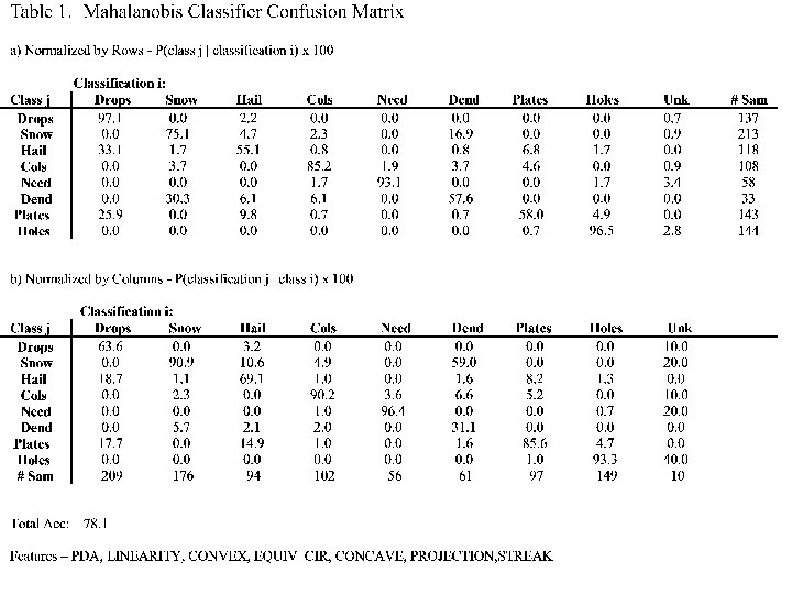
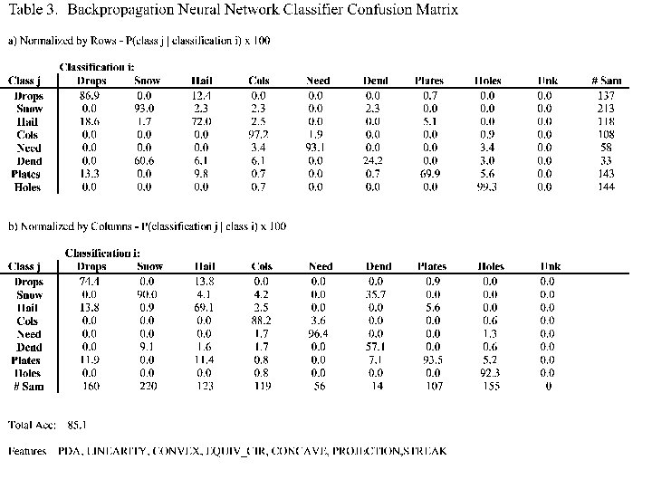
Features selected • PDA – Perimeter Diameter Area (PDA) – The product of the perimeter and diameter divided by the area. Smooth, circular images give smaller values while irregular ones give larger values. • Linearity – The correlation coefficient for the regression. Values for linear images, such as of a needle or column, are closer to 1. This is as opposed to circularly symmetric images that have values closer to 0. A Holroyd measure. • equivalent circle – Equivalent Circle – The diameter of a circle that has the same area as the particle image.

Features selected • Concavity – The ratio of the number of concave perimeter points to the distance around the convex hull. Convex images give zero or small values while images with concavities give larger values. • projection fit - The standard error of a least squares quadratic regression of the projection of the number of pixels in the vertical along the horizontal. Smooth, circular images give low standard errors while irregular shapes give high errors.

Features selected • convex hull – The convex hull is the distance around the perimeter of a particle image as though a rubber band were stretched around it, or the distance traversed by rolling the image along a straight line.

Feature Distributions • Distributions are not always: – Gaussian – Monomodal – Well separated between/among classes

Classification Methodologies • Mahalanobis Minimum Distance • Fuzzy Logic • Backpropagation Neural Network

Mahalanobis • Form of Maximum Likelihood Classifier – Assume equal a priori probabilities – A Euclidean distance with directionality Richards, 1986

Mahalanobis (2 D feature space) Probability of image belonging to each P class Class 1 Feature 1 Class 2 Class 3 Feature 2 Richards, 1986

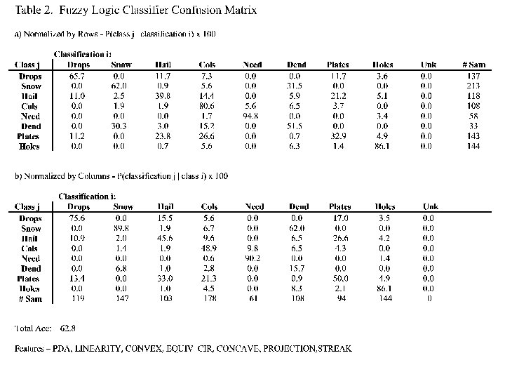
Results • Performance or accuracy of each of 3 classifiers was derived using a separate set of training and testing sample images

Confusion Matrices

What is the best classification methodology?

Conclusions • For these samples, BPNN provides best performance; however, MMDC is a close second • Feature set selection is tantamount to classifier selection