Those who dont know statistics are condemned to

Those who don’t know statistics are condemned to reinvent it… David Freedman

All you ever wanted to know about the histogram and more. . .

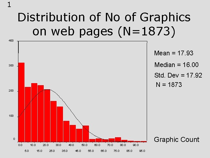
1 Distribution of No of Graphics on web pages (N=1873) 400 Mean = 17. 93 Median = 16. 00 300 Std. Dev = 17. 92 N = 1873 200 100 Graphic Count 0 0. 0 10. 0 5. 0 20. 0 15. 0 30. 0 25. 0 40. 0 35. 0 50. 0 45. 0 60. 0 55. 0 70. 0 65. 0 80. 0 75. 0 90. 0 85. 0 95. 0

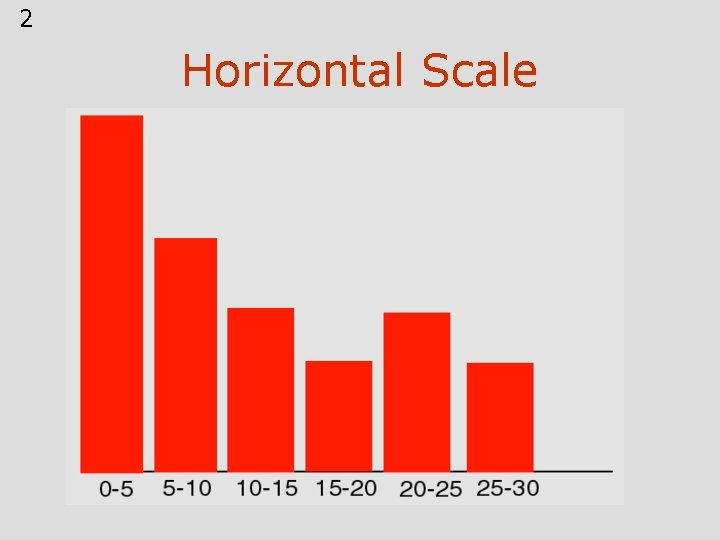
2 Horizontal Scale

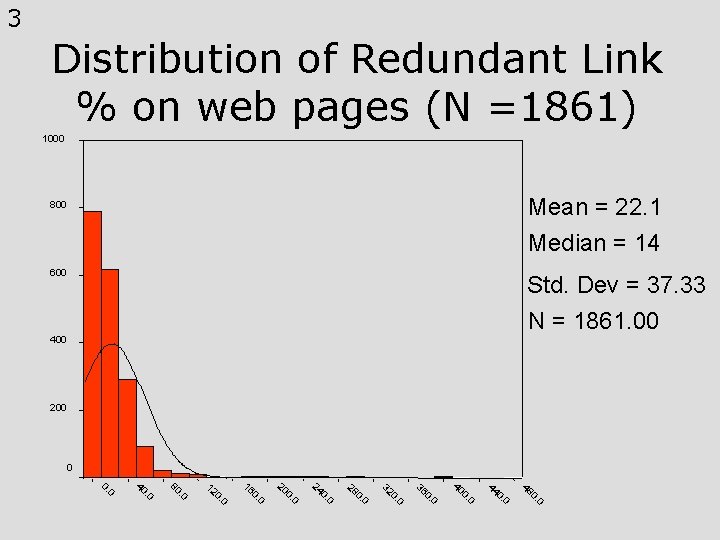
3 Distribution of Redundant Link % on web pages (N =1861) 1000 Mean = 22. 1 Median = 14 800 600 Std. Dev = 37. 33 N = 1861. 00 400 200 0 0 0. 48 0 0. 44 0 0. 40 0 0. 36 0 0. 32 0 0. 28 0 0. 24 0 0. 20 0 0. 16 0 0. 12 . 0 80 . 0 40 0 0.

Plotting a histogram: endpoint convention, plot frequencies, make equal intervals etc.

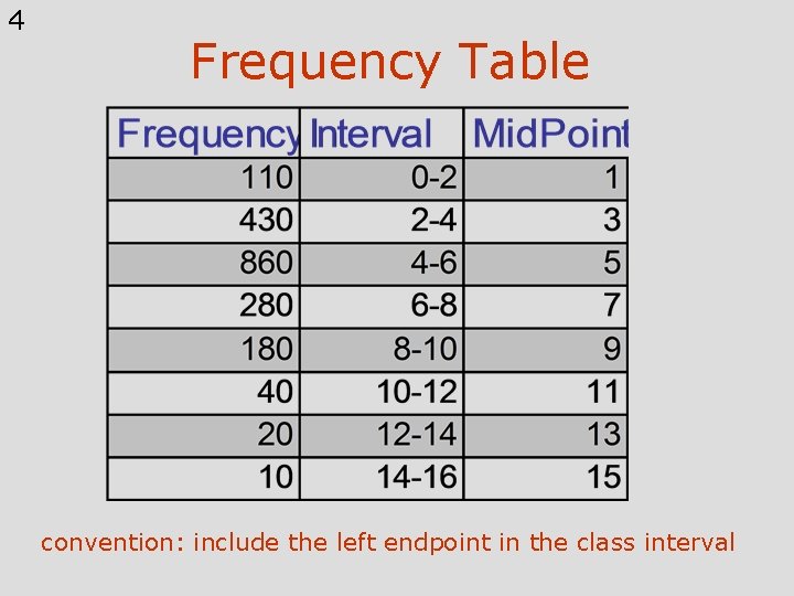
4 Frequency Table convention: include the left endpoint in the class interval

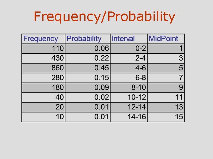
Frequency/Probability

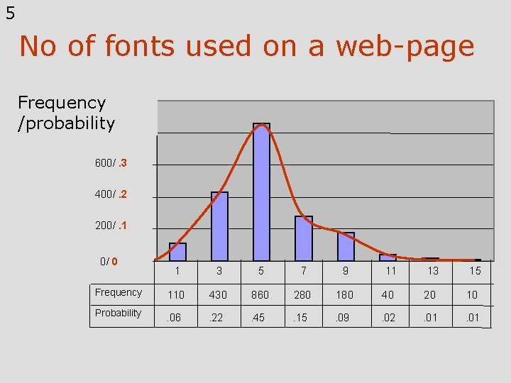
5 No of fonts used on a web-page 1000/. 5 Frequency /probability 800/. 4 600/. 3 400/. 2 200/. 1 0/ 0 1 3 5 7 9 11 13 15 Frequency 110 430 860 280 180 40 20 10 Probability . 06 . 22 . 45 . 15 . 09 . 02 . 01

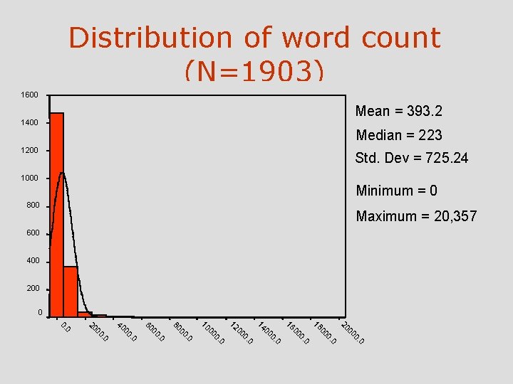
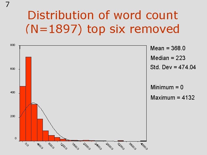
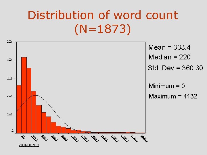
Cleaning up a histogram: getting rid of outliers

Distribution of word count (N=1903) 1600 Mean = 393. 2 1400 Median = 223 1200 Std. Dev = 725. 24 1000 Minimum = 0 800 Maximum = 20, 357 600 400 200 0 00 20 . 0 0 00 18. 0 0 00 16 0 0. 00 14 0 0. 00 12 0 0 0. 00 10 . 00 80 0 . 00 60 . 00 40 . 00 20 0 0.

7 Distribution of word count (N=1897) top six removed 800 Mean = 368. 0 Median = 223 Std. Dev = 474. 04 600 Minimum = 0 400 Maximum = 4132 200 0 . 0 00 40 . 0 00 36 . 0 00 32. 0 00 28. 0 00 24 . 0 00 20. 0 00 16 . 0 00 12 0 0. 80 0 0. 40 0 0.

Distribution of word count (N=1873) 500 Mean = 333. 4 Median = 220 400 Std. Dev = 360. 30 300 Minimum = 0 Maximum = 4132 200 100 0. 0 00 24 . 0 00 22 . 0 00 20 . 0 00 18 . 0 00 16 . 0 00 14 . 0 00 12 . 0 00 10 0 0. 80 0 0. 60 0 0. 40 0 0. 20 0 0. WORDCNT 2

What can histograms tell you

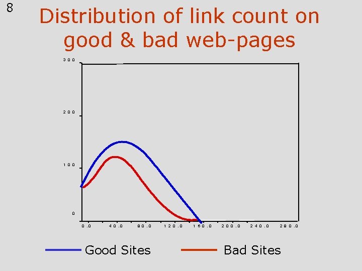
8 Distribution of link count on good & bad web-pages 3 0 0 2 0 0 1 0 0. 0 4 0. 0 8 0. 0 Good Sites 1 2 0. 0 1 6 0. 0 2 0 0. 0 2 4 0. 0 2 8 0. 0 Bad Sites

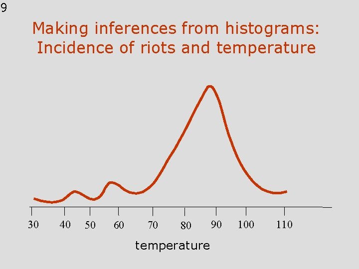
9 Making inferences from histograms: Incidence of riots and temperature 30 40 50 60 70 80 temperature 90 100 110

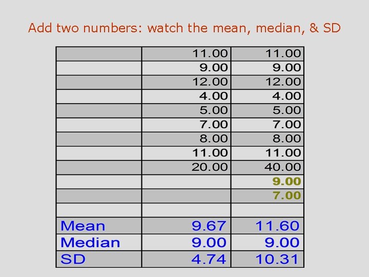
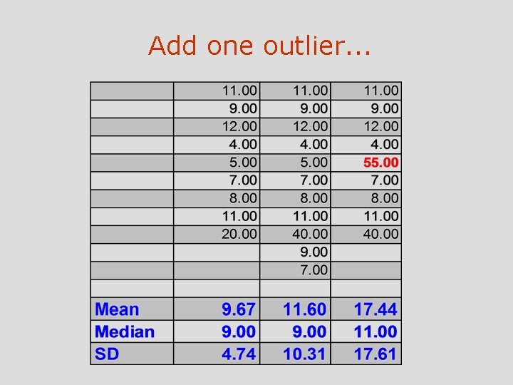
Mean and Median Mean is arithmetic average, median is 50% point Mean is point where graph balances Mean shifts around, Median does not shift much, is more stable Computing Median: for odd numbered N find middle number For even numbered N interpolate between middle 2, e. g. if it is 7 and 9, then 8 is the median

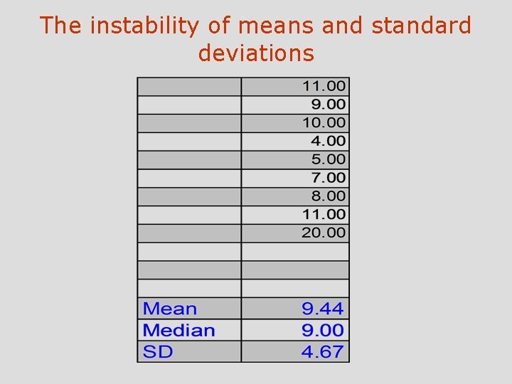
The instability of means and standard deviations

Add two numbers: watch the mean, median, & SD

Add one outlier. . .

Standard Deviation: a measure of spread

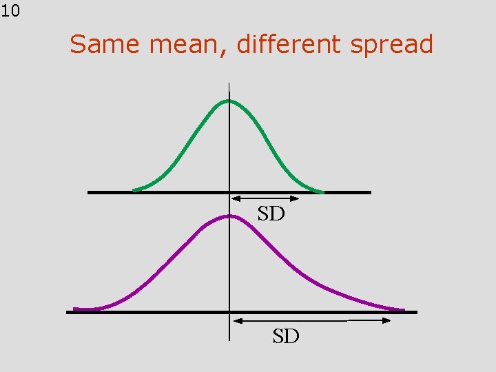
10 Same mean, different spread SD SD

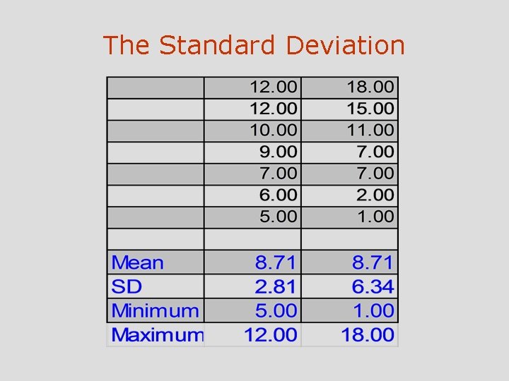
The Standard Deviation

The SD says how far away numbers on a list are from their average. Most entries on the list will be somewhere around one SD away from the average. Very few will be more than two or three SD’s away.

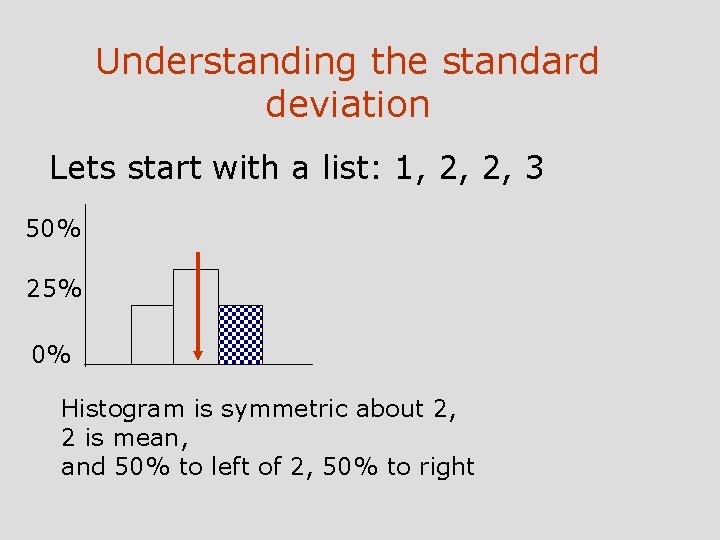
Understanding the standard deviation Lets start with a list: 1, 2, 2, 3 50% 25% 0% Histogram is symmetric about 2, 2 is mean, and 50% to left of 2, 50% to right

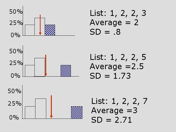
50% 25% 0% List: 1, 2, 2, 3 Average = 2 SD =. 8 List: 1, 2, 2, 5 Average =2. 5 SD = 1. 73 50% 25% 0% List: 1, 2, 2, 7 Average =3 SD = 2. 71

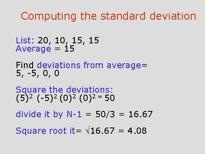
Computing the standard deviation List: 20, 15, 15 Average = 15 Find deviations from average= 5, -5, 0, 0 Square the deviations: (5)2 (-5)2 (0)2 = 50 divide it by N-1 = 50/3 = 16. 67 Square root it= 16. 67 = 4. 08

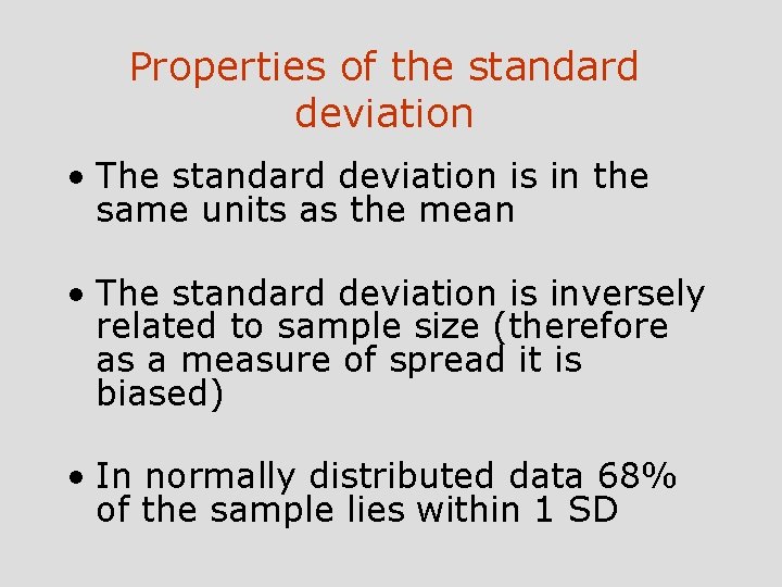
Properties of the standard deviation • The standard deviation is in the same units as the mean • The standard deviation is inversely related to sample size (therefore as a measure of spread it is biased) • In normally distributed data 68% of the sample lies within 1 SD

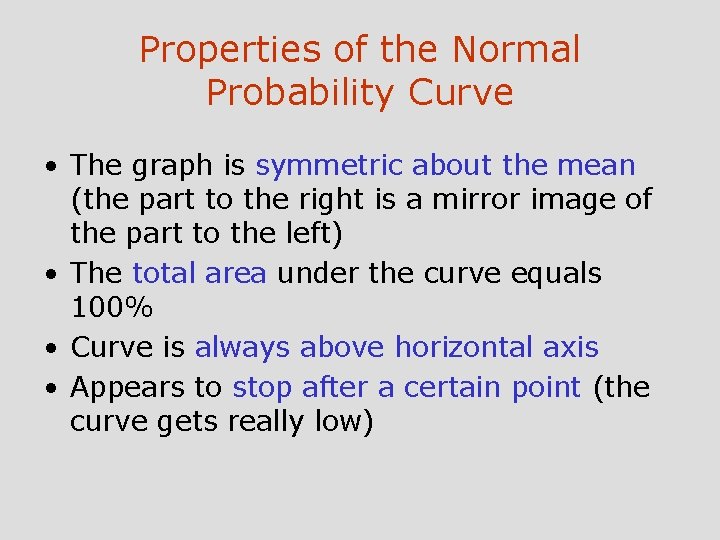
Properties of the Normal Probability Curve • The graph is symmetric about the mean (the part to the right is a mirror image of the part to the left) • The total area under the curve equals 100% • Curve is always above horizontal axis • Appears to stop after a certain point (the curve gets really low)

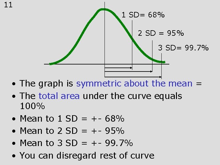
11 1 SD= 68% 2 SD = 95% 3 SD= 99. 7% • The graph is symmetric about the mean = • The total area under the curve equals 100% • Mean to 1 SD = +- 68% • Mean to 2 SD = +- 95% • Mean to 3 SD = +- 99. 7% • You can disregard rest of curve

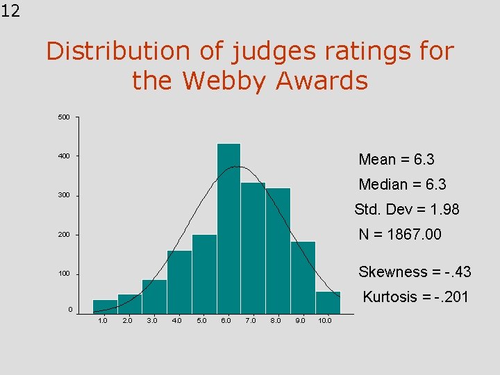
12 Distribution of judges ratings for the Webby Awards 500 Mean = 6. 3 400 Median = 6. 3 300 Std. Dev = 1. 98 200 N = 1867. 00 100 Skewness = -. 43 Kurtosis = -. 201 0 1. 0 2. 0 3. 0 4. 0 5. 0 6. 0 7. 0 8. 0 9. 0 10. 0

It is a remarkable fact that many histograms in real life tend to follow the Normal Curve. For such histograms, the mean and SD are good summary statistics. The average pins down the center, while the SD gives the spread. For histogram which do not follow the normal Curve, the mean and SD are not good summary statistics. What when the histogram is not normal. . .

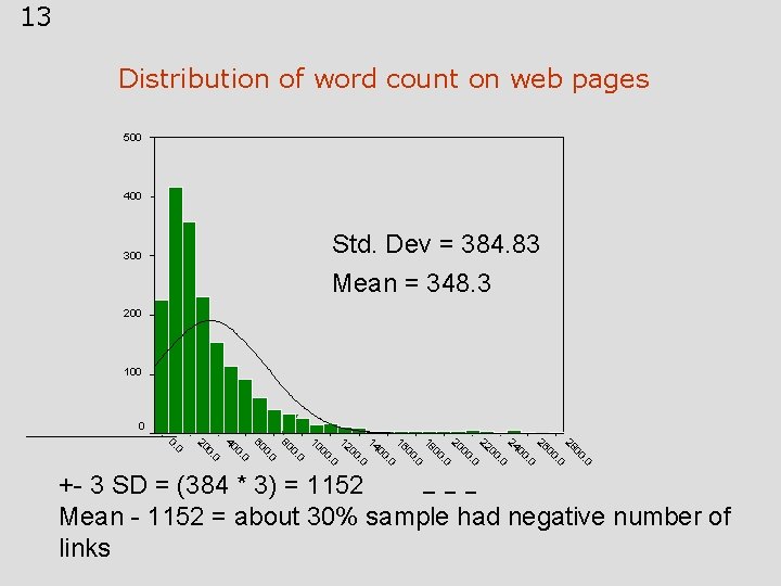
13 Distribution of word count on web pages 500 400 Std. Dev = 384. 83 Mean = 348. 3 300 200 100 0. 0 00 28. 0 00 26. 0 00 24. 0 00 22. 0 00 20. 0 00 18. 0 00 16. 0 00 14. 0 00 12 . 0 00 10 0 0. 80 0 0. 60 0 0. 40 0 0. 20 0 0. +- 3 SD = (384 * 3) = 1152 Mean - 1152 = about 30% sample had negative number of links

When SD is influenced by outliers Use inter quartile range 75 th percentile - 25 th percentile Note. A percentile is a score below which a certain % of sample is

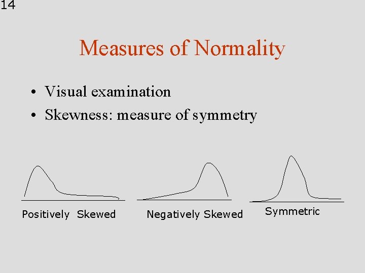
14 Measures of Normality • Visual examination • Skewness: measure of symmetry Positively Skewed Negatively Skewed Symmetric

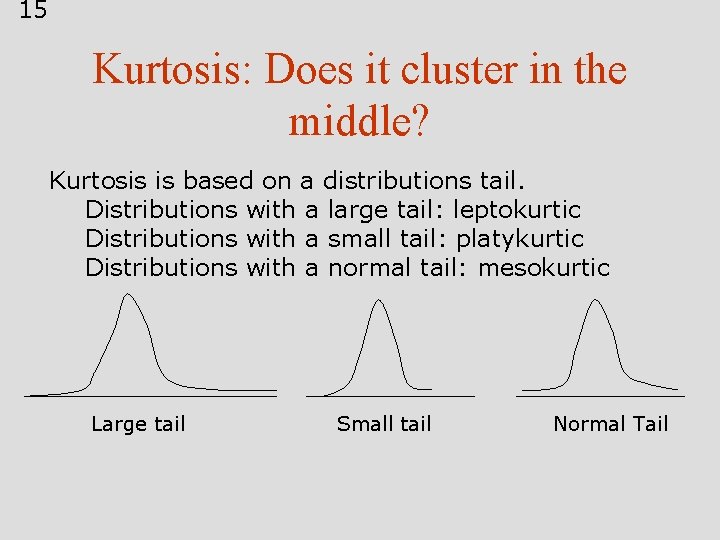
15 Kurtosis: Does it cluster in the middle? Kurtosis is based on a distributions tail. Distributions with a large tail: leptokurtic Distributions with a small tail: platykurtic Distributions with a normal tail: mesokurtic Large tail Small tail Normal Tail

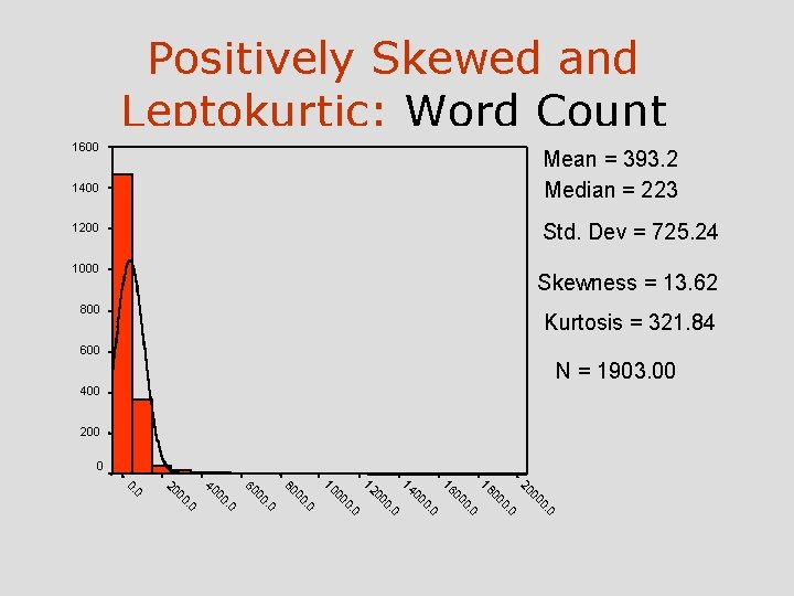
Positively Skewed and Leptokurtic: Word Count 1600 Mean = 393. 2 Median = 223 1400 Std. Dev = 725. 24 1200 1000 Skewness = 13. 62 800 Kurtosis = 321. 84 600 N = 1903. 00 400 200 0 0 . 0 0. 00 20 0 00 18 0. 00 16 0. 00 14 0 . 0 0 00 12 0 0. 00 10 . 00 80 0 . 00 60 . 00 40 . 00 20 0 0.

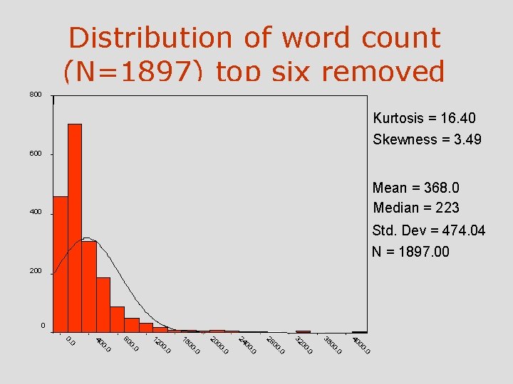
Distribution of word count (N=1897) top six removed 800 Kurtosis = 16. 40 Skewness = 3. 49 600 Mean = 368. 0 Median = 223 400 Std. Dev = 474. 04 N = 1897. 00 200 0. 0 00 40 . 0 00 36 . 0 00 32 . 0 00 28 . 0 00 24 . 0 00 20 . 0 00 16 . 0 00 12 0 0. 80 0 0. 40 0 0.

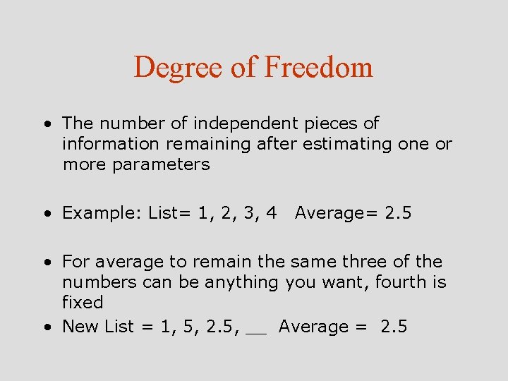
Degree of Freedom • The number of independent pieces of information remaining after estimating one or more parameters • Example: List= 1, 2, 3, 4 Average= 2. 5 • For average to remain the same three of the numbers can be anything you want, fourth is fixed • New List = 1, 5, 2. 5, __ Average = 2. 5