This Week Review of estimation and hypothesis testing

This Week • Review of estimation and hypothesis testing • Reading Le (review) – Chapter 4: Sections 4. 1 – 4. 3 – Chapter 5: Sections 5: 1 and 5: 4 – Chapter 7: Sections 7: 1 – 7. 3 • Reading C &S – Chapter 2: A-E – Chapter 6: A, B, F

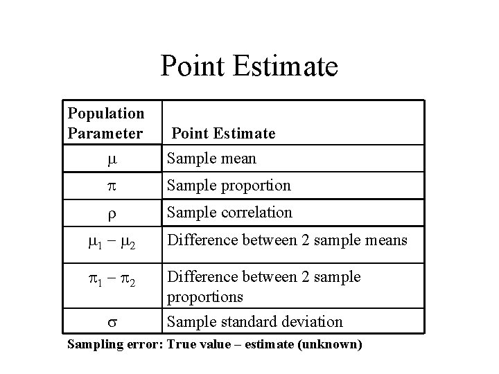
Point Estimate Population Parameter Point Estimate m Sample mean p Sample proportion r Sample correlation m 1 - m 2 Difference between 2 sample means p 1 - p 2 Difference between 2 sample proportions Sample standard deviation s Sampling error: True value – estimate (unknown)

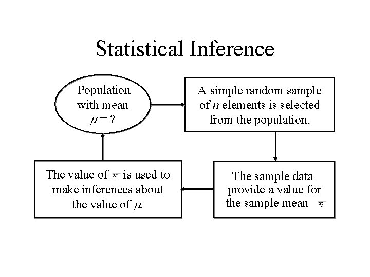
Statistical Inference Population with mean m=? The value of is used to make inferences about the value of m. A simple random sample of n elements is selected from the population. The sample data provide a value for the sample mean.

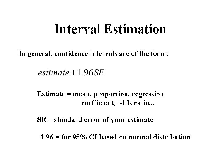
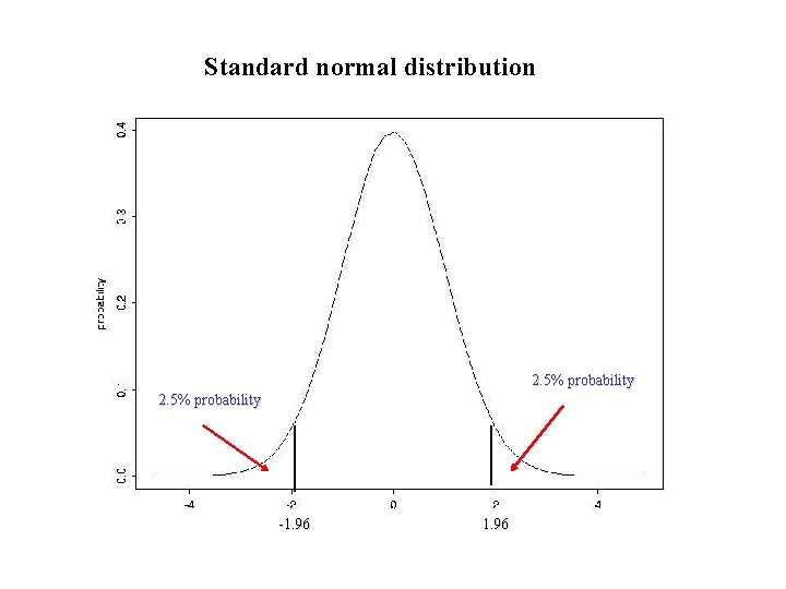
Interval Estimation In general, confidence intervals are of the form: Estimate = mean, proportion, regression coefficient, odds ratio. . . SE = standard error of your estimate 1. 96 = for 95% CI based on normal distribution

Standard normal distribution 2. 5% probability -1. 96

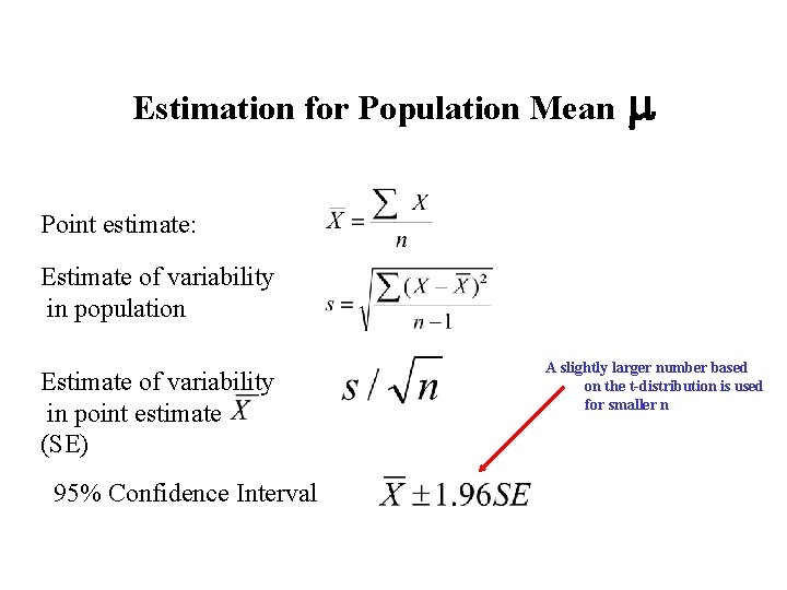
Estimation for Population Mean m Point estimate: Estimate of variability in population Estimate of variability in point estimate (SE) 95% Confidence Interval A slightly larger number based on the t-distribution is used for smaller n

Assumptions • Data in population follows a normal distribution or • Sample size is large enough to apply central limit theorem (CLT) • CLT – no matter the shape of the population distribution of the sample mean approaches a normal distribution as the sample size gets large

Meaning of Confidence Interval • There is a 95% chance that your interval contains m. (That you “captured” the true value m with your interval)

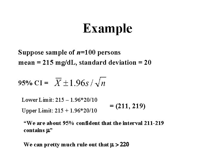
Example Suppose sample of n=100 persons mean = 215 mg/d. L, standard deviation = 20 95% CI = Lower Limit: 215 – 1. 96*20/10 Upper Limit: 215 + 1. 96*20/10 = (211, 219) “We are about 95% confident that the interval 211 -219 contains m” We can pretty much rule out that m > 220

Properties of Confidence Intervals • As sample size increases, CI gets smaller – Because SE gets smaller; • Can use different levels of confidence – 90, 95, 99% common – More confidence means larger interval; so a 90% CI is smaller than a 99% CI – What would a 100% CI look like? • Changes with population standard deviation – More variable population means larger interval

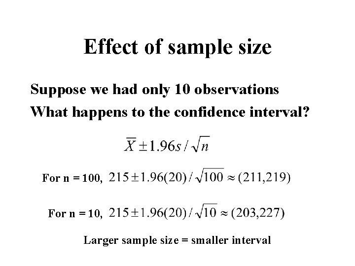
Effect of sample size Suppose we had only 10 observations What happens to the confidence interval? For n = 100, For n = 10, Larger sample size = smaller interval

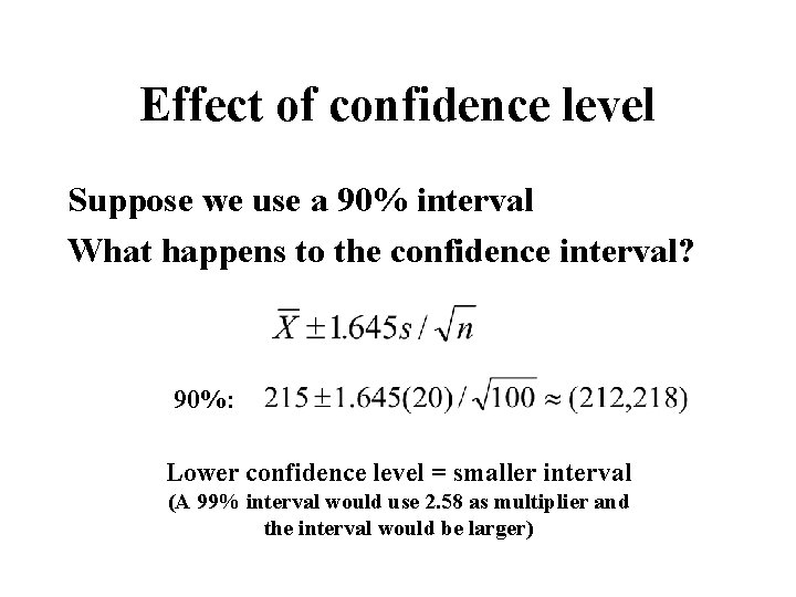
Effect of confidence level Suppose we use a 90% interval What happens to the confidence interval? 90%: Lower confidence level = smaller interval (A 99% interval would use 2. 58 as multiplier and the interval would be larger)

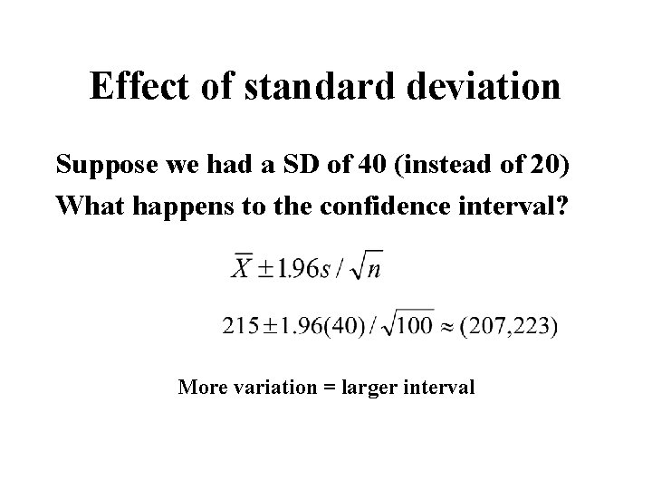
Effect of standard deviation Suppose we had a SD of 40 (instead of 20) What happens to the confidence interval? More variation = larger interval

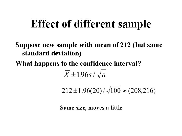
Effect of different sample Suppose new sample with mean of 212 (but same standard deviation) What happens to the confidence interval? Same size, moves a little

How Big A Sample To Take? • Depends on the variability in the population • Depends on how precise an estimate you want • Cost - if it doesn’t cost much to sample an element then sample many

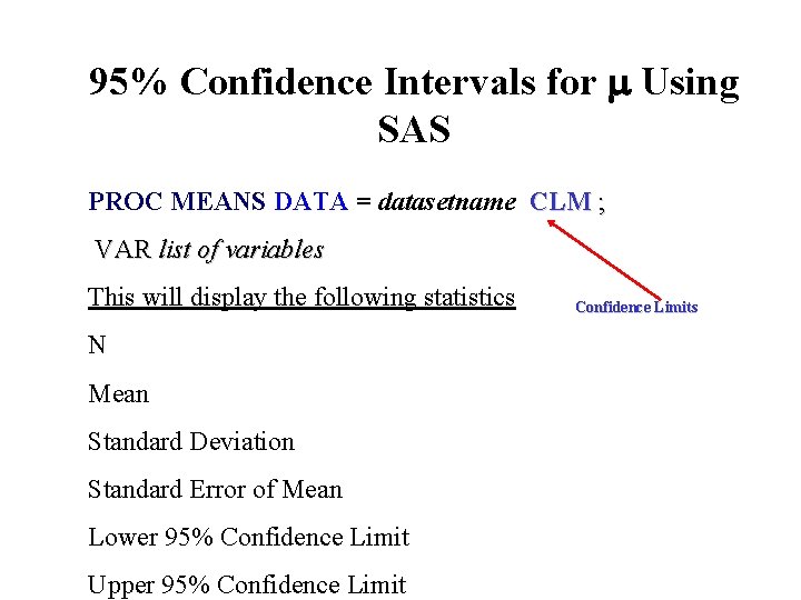
95% Confidence Intervals for m Using SAS PROC MEANS DATA = datasetname CLM ; VAR list of variables This will display the following statistics N Mean Standard Deviation Standard Error of Mean Lower 95% Confidence Limit Upper 95% Confidence Limits

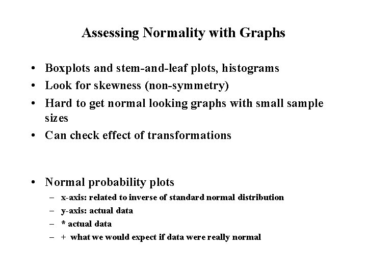
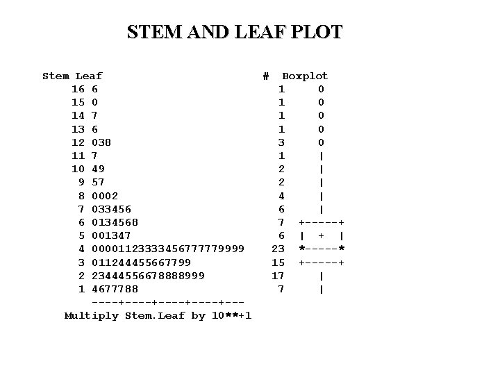
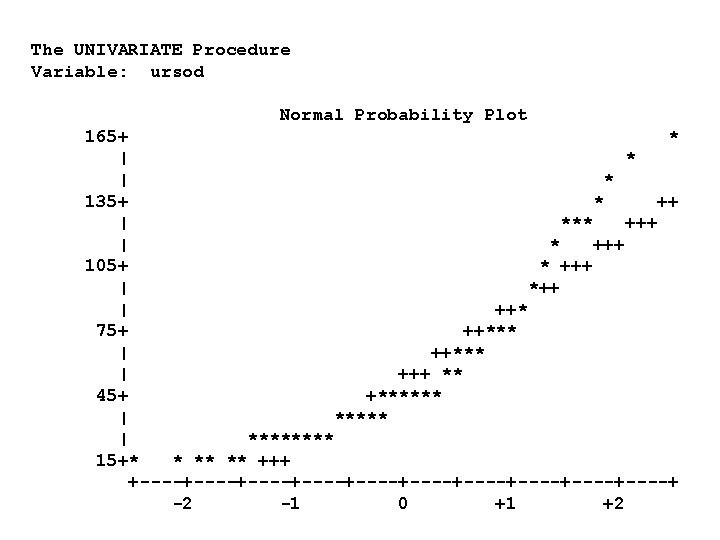
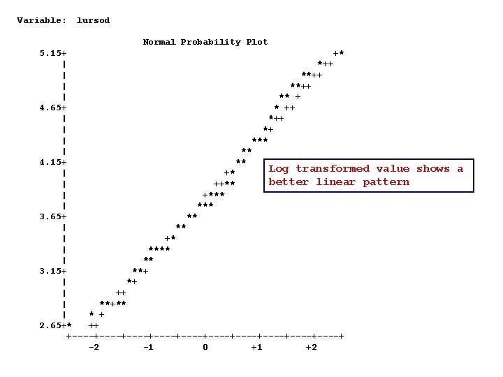
Assessing Normality with Graphs • Boxplots and stem-and-leaf plots, histograms • Look for skewness (non-symmetry) • Hard to get normal looking graphs with small sample sizes • Can check effect of transformations • Normal probability plots – – x-axis: related to inverse of standard normal distribution y-axis: actual data * actual data + what we would expect if data were really normal

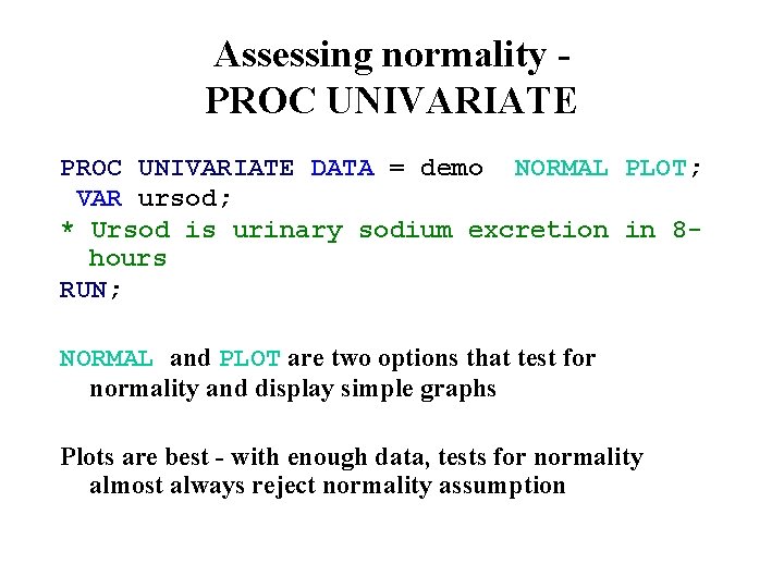
Assessing normality PROC UNIVARIATE DATA = demo NORMAL PLOT; VAR ursod; * Ursod is urinary sodium excretion in 8 hours RUN; NORMAL and PLOT are two options that test for normality and display simple graphs Plots are best - with enough data, tests for normality almost always reject normality assumption

STEM AND LEAF PLOT Stem Leaf # Boxplot 16 6 1 0 15 0 14 7 1 0 13 6 1 0 12 038 3 0 11 7 1 | 10 49 2 | 9 57 2 | 8 0002 4 | 7 033456 6 | 6 0134568 7 +-----+ 5 001347 6 | + | 4 00001123333456777779999 23 *-----* 3 011244455667799 15 +-----+ 2 23444556678888999 17 | 1 4677788 7 | ----+----+--Multiply Stem. Leaf by 10**+1

The UNIVARIATE Procedure Variable: ursod Normal Probability Plot 165+ * | * 135+ * ++ | *** +++ | * +++ 105+ * +++ | *++ | ++* 75+ ++*** | +++ ** 45+ +****** | **** 15+* * ** ** +++ +----+----+----+----+----+ -2 -1 0 +1 +2

Variable: lursod Normal Probability Plot 5. 15+ +* | *++ | **++ | ** + 4. 65+ * ++ | *+ | *** | ** 4. 15+ ** Log transformed value | +* better linear pattern | ++** | +*** | *** 3. 65+ ** | +* | **** | ** 3. 15+ **+ | ++ | **+** | * + 2. 65+* ++ +----+----+----+----+----+ -2 -1 0 +1 +2 shows a

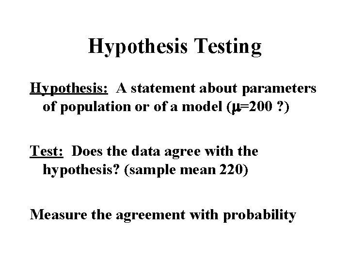
Hypothesis Testing Hypothesis: A statement about parameters of population or of a model (m=200 ? ) Test: Does the data agree with the hypothesis? (sample mean 220) Measure the agreement with probability

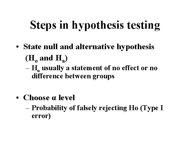
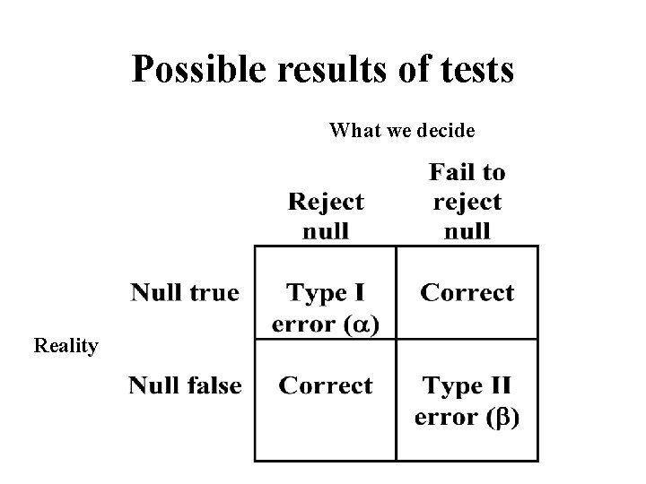
Steps in hypothesis testing • State null and alternative hypothesis (Ho and Ha) – Ho usually a statement of no effect or no difference between groups • Choose α level – Probability of falsely rejecting Ho (Type I error)

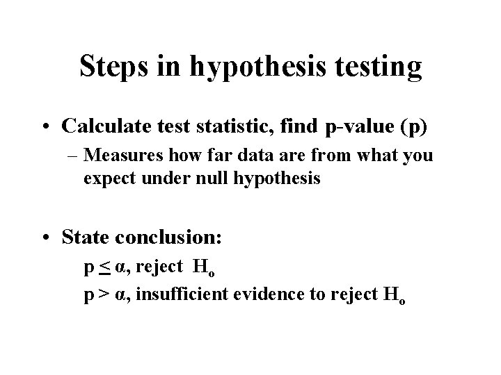
Steps in hypothesis testing • Calculate test statistic, find p-value (p) – Measures how far data are from what you expect under null hypothesis • State conclusion: p < α, reject Ho p > α, insufficient evidence to reject Ho

Possible results of tests What we decide Reality

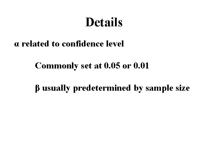
Details α related to confidence level Commonly set at 0. 05 or 0. 01 β usually predetermined by sample size

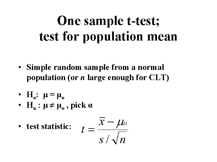
One sample t-test; test for population mean • Simple random sample from a normal population (or n large enough for CLT) • Ho: μ = μo • Ha : μ μo , pick α • test statistic:

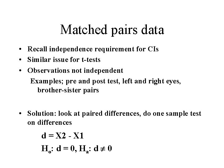
Matched pairs data • Recall independence requirement for CIs • Similar issue for t-tests • Observations not independent Examples; pre and post test, left and right eyes, brother-sister pairs • Solution: look at paired differences, do one sample test on differences d = X 2 - X 1 Ho: d = 0, Ha: d 0

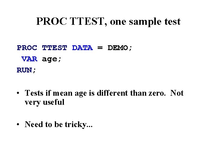
PROC TTEST, one sample test PROC TTEST DATA = DEMO; VAR age; RUN; • Tests if mean age is different than zero. Not very useful • Need to be tricky. . .

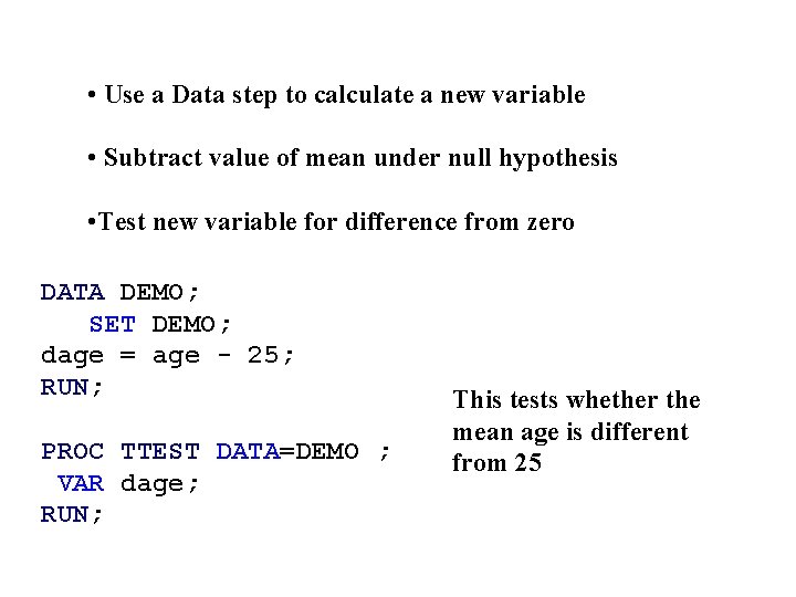
• Use a Data step to calculate a new variable • Subtract value of mean under null hypothesis • Test new variable for difference from zero DATA DEMO; SET DEMO; dage = age - 25; RUN; PROC TTEST DATA=DEMO ; VAR dage; RUN; This tests whether the mean age is different from 25

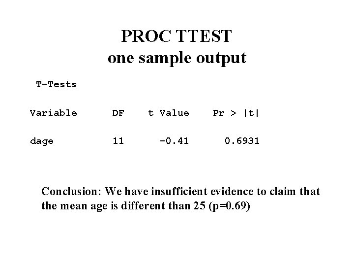
PROC TTEST one sample output T-Tests Variable DF t Value Pr > |t| dage 11 -0. 41 0. 6931 Conclusion: We have insufficient evidence to claim that the mean age is different than 25 (p=0. 69)