This slide is intentionally blank What is PerpleX

This slide is intentionally blank

What is Perple_X doing? Constrained Gibbs Energy Minimization Unconstrained Gibbs Energy Minimization Iteration, and Iteration…

Constrained Gibbs Energy Minimization * The pressure, temperature, and composition of the system is specified and the stable phases are predicted Key assumptions: Bulk equilibrium – no mineral zoning, no retrograde minerals, etc. The mineralogical models describe all important solution behavior – e. g. if Zn is a component, then Zn solution must be described in every phase in which it is a potentially important constituent *Perple_X programs VERTEX and MEEMUM

Constrained Gibbs Energy Minimization The stable state of a system minimizes its Gibbs Energy (G)

Non-Linear Gibbs Energy minimization Brown & Skinner 1974, Saxena & Eriksson 1983, Wood & Holloway 1984, de. Capitani & Brown 1987, Bina 1998, etc. , see Connolly 2017 for a review of petrologic optimization schemes

Linear Gibbs Energy Minimization

Linearized Gibbs Energy Minimization: “Pseudocompound” Approximation Pseudocompounds White et al. , 1958; Connolly & Kerrick 1987
 The Problem with Pseudocompounds The solution =>")
Iteration Scheme #1: Adaptive Minimization (Connolly 2009) The Problem with Pseudocompounds The solution => iteration Relevant Perple_X options: initial_resolution, final_resolution, resolution_factor, refinement_points, reach_increment. See: www. perplex. ethz. ch/Perple_X_why_it_often_does_not_work. html
 phase diagrams are hyperdimensional objects. Fortunately in many cases we require")
In general (c>1) phase diagrams are hyperdimensional objects. Fortunately in many cases we require only information in 1 -, 2 -, or 3 -dimensional phase diagram or phase diagram section. In such cases phase diagram construction can be thought of as a mapping problem in which Gibbs energy minimization is tool used for sampling.
")
Phase diagram sections as a mapping problem Iteration Scheme #2: Gridded Minimization (Connolly 2005) Oval object to be mapped The final map The problem is analogous to mapping an oval rock exposure except that in the case of a phase field the identification of the phase assemblage at any sampling point is determined by the accuracy of the adapative minimization procedure (Iteration Scheme #1), i. e. , there is no value to high resolution mapping with low resolution minimization. Balancing the resolution of both schemes is one of the many challenges to using Perple_X efficiently. Relevant Perple_X options: 1 d_path, x_nodes, y_nodes, grid_levels

Iteration Scheme #3: Auto-refinement By default Perple_X does every calculation twice: a low-resolution exploratory stage and a high-resolution auto-refine stage After the exploratory stage Perple_X: 1) eliminates unstable solution models 2) restricts the compositional range of stable solution models 3) increases the resolution of the adaptive and gridded minimization schemes* Relevant Perple_X options: auto_refine, reach_increment_switch *the following options have different values for the exploratory and auto-refine stage: initial_resolution, final_resolution, resolution_factor, refinement_points, reach_increment_switch, x_nodes, y_nodes, 1 d_path, grid_levels See: www. perplex. ethz. ch/Perple_X_why_it_often_does_not_work. html

Constrained minimization can easily be used to treat path-dependent problems such as phase fractionation and reactive-transport An Example: Subduction Zone Decarbonation (Connolly 2005*) Closed system models suggest carbonates in slab lithologies remain stable beyond sub-arc depths (Kerrick & Connolly, 1998, 2001 a, b). Would infiltration-driven decarbonation alter this conclusion? *Input for this type of calculation is documented at: www. perplex. ethz. ch/Perple_X_FRAC 2 D. html
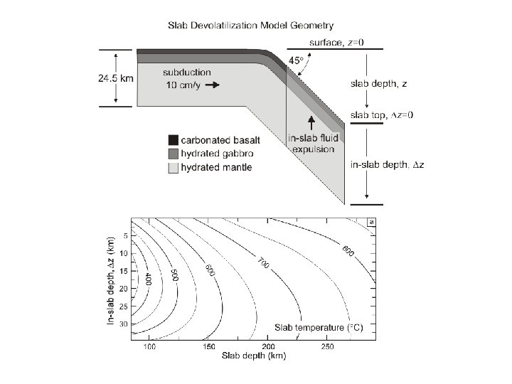


Slab fluid composition and production

Slab Properties Is infiltration decarbonation important? No. Taras Gerya is probably right!

What if you add electrolytes? Maybe… *The input for this type of calculation, 0 -D infiltration/fractionation, is at: www. perplex. ethz. ch/perplex_electrolyte. html#Files_for_Connolly_2018
* All possible compositions of the system are optimized")
Unconstrained Gibbs Energy Minimization (Connolly 1990)* All possible compositions of the system are optimized simultaneously Key advantages: No assumption of bulk equilibrium, complete solution models are not critical Permits classical phase petrological phase diagram constructions: chemographic analysis, isopotential phase diagram sections, Schreinemakers projections Key disadvantages: Limited resolution, complexity *Perple_X program CONVEX

The Linear Convexhull Problem A B

The Linearized Convexhull Problem: “Pseudocompound” Approximation Pseudocompounds Connolly & Kerrick 1987
 The plot on the right is")
An Example: CAS after Berman & Brown (1984) The plot on the right is the default plot from PSVDRAW, the plot on the left which shows the vertices of the convexhull (i. e. , the stable pseudocompounds) is obtained from PSVDRAW, by modifying the default to plot “tielines”.

Why is there a choice? VERTEX - Linear Programming CONVEX - Convexhull The plot on the right is the default plot from PSVDRAW, the plot on the left is obtained with PSSECT. Currently PSSECT offers no provision to transform the orthogonal compositional coordinates to the coordinate system of the equilateral triangle commonly used to represent ternary compositions.

An Example: Schreinemakers Projection for C-saturated ultramafic rocks as a function of temperature and fluid composition

A bit of “theory”
 diagram")
What is a phase diagram? A phase diagram is a (real or abstract) diagram that directly defines the relative amounts and state of the phases in a thermodynamic system

What is state? State is thermal, mechanical, and chemical configuration of matter without regard to its size (extent) In a system with k chemical kinds of mass, there are k+2 independent thermodynamic variables, but there are only k+1 independent state variables There are two types of state variables Potential variables - (P, T, chemical potentials*) do not differ among the coexisting phases of an equilibrium system Specific variables - (s, v, chemical compositions) differ among the coexisting phases of an equilibrium system The state of a p-phase system is only defined in a phase diagram with n ≥ p-1 specific variables *Variables such as the composition of a phase (e. g. , X CO 2 in binary H 2 O-CO 2 fluids) or the properties of a hypothetical species (e. g. , f O 2, Eh, p. H, etc) are an indirect means of specifying chemical potentials. They are therefore classified as potential variables (Connolly 1990, Connolly & Petrini 2002).

Thermodynamic and Phase Diagram Variables* *…, Tisza 1966, Callen 1981, Hillert 1986, …, Connolly 1990, …
 s (adiabatic) Mechanical P (inviscid) v")
Variable Choices Environment/Intensiv e System/Extensive Thermal T (diathermal) s (adiabatic) Mechanical P (inviscid) v (isochoric) Chemical m (mobile) M (inert) Phase diagrams are most useful when the variables of the phase diagram correspond to the determinative variables of the physicochemical system of interest. The observation of a phase assemblage that corresponds to an indefinite state (i. e. , a heterogeneous reaction) in a phase diagram indicates that the variables of the phase diagram do not correspond to the determinative variables of the system. E. g. , observation of the equilibrium assemblage kyanite + andalusite indicates that pressure and temperature cannot have been truly determinative variables, i. e. , the reaction kyanite = andalusite must have influenced (aka buffered) pressure and/or temperature.

Changing Variables P, T – state defined for p = 1 v, T – state defined for p ≤ 2 P, s – state defined for p ≤ 2 v, s – state defined for p ≤ 3 *…, Korzskii (1959), JB Thompson (the American Petrological renaissance ~1975), Hillert (1986), …, Connolly (1990), …

What does a calculated s-v phase diagram look like?

Reducing Multidimensional Phase Diagrams to 2 D Can be constructed with CONVEX

Reducing Multidimensional Phase Diagrams to 2 D AKA Mixed-variable phase diagrams Can be constructed with CONVEX or VERTEX (can be non-linear, e. g. , P(T))

Reducing Multidimensional Phase Diagrams to 2 D AKA pseudosections (the term is nonsense, isochemical sections are pseudo-phase diagrams not pseudo-sections) Value: defines exact phase stabilities for a specific bulk composition Can be constructed with VERTEX

Reducing Multidimensional Phase Diagrams to 2 D AKA Petrogenetic grids Value: defines absolute phase stabilities irrespective of bulk composition Can be constructed with CONVEX It is often suggested that the projected axes of a Schreinemakers’ Projection correspond to composition variables. There is no such constraint, i. e. , the projection is identical if a compositional variable or its conjugate potential corresponds to a projected axes. Additionally, the Schreinemakers’ Projection is equally valid if pressure (or volume) or temperature (or entropy) correspond to the projected axes (Connolly 1990).

If you got this far, you might as well know the truth… “Phase diagrams are the beginning of wisdom not the end of it. ” -- Sir William Hume-Rothery Good luck!
men to lose hours like slaves in the labor")
“It is unworthy of great (wo)men to lose hours like slaves in the labor of calculation. ” -- Baron Gottfried Wilhelm von Leibniz Perple_X : A Mechanical Petrologist for Geophysical Problems What is Perple_X doing? Geophysical inversion for mantle composition and temperature A few thoughts about nomenclature

The Non-Linear Phase Equilibrium Problem The stable state of a system minimizes its Gibbs Energy (G)

The Non-Linear Phase Equilibrium Problem The stable state of a system minimizes its Gibbs Energy (G) Brown & Skinner 1974, Saxena & Eriksson 1983, Wood & Holloway 1984, de. Capitani & Brown 1987, Bina 1998, etc.

Iteration Scheme #1: Adaptive Minimization The Problem with Pseudocompounds The solution => iteration White et al. 1958, Connolly 2009

What if the bulk composition is known? Pseudocompounds White et al. 1958, Connolly 2005

A Problem with Pseudocompounds White et al. 1958, Connolly 2009 A Solution: Iterative Refinement

Phase diagram sections as a mapping problem
 Linear Programming Convex")
An Example: Again CAS after Berman & Brown (1984, no comment) Linear Programming Convex Hull

What is a phase diagram? A phase diagram is any diagram that directly defines the relative amounts and state of the phases in a thermodynamic system Phase diagram variables vs real determinative variables

The advantage of LP is it permits melts of natural complexity An example: Peridotite solidus with the p. MELTS model (Ghiorso et al. 2003)

Conclusions for Part I But a monkey could do that… The beginning of wisdom? Putting phase equilibria (g) into geophysics…

Equation of State, Stixrude & Bukowinski 1990 Gruneisen model for Helmoltz Energy: Birch-Murgnahan “cold” part: Debeye “thermal” part: Seven parameters ( ) + 3 parameters for seismic velocities Data from Stixrude & Lithgow-Bertelloni (2005) augmented by • Post-perovskite from Oganov & Ono (2004), Ono & Oganov (2005) • Ca-perovskite from Akaogi et al. (2004), Karki & Crain (1998) • Wuestite, perovskite from Fabrichnaya (1999), Irifune (1994)
 Phase Relations")
Computed Pyrolite (Ca. O-Fe. O-Mg. O-Al 2 O 3 -Si. O 2) Phase Relations

Pyrolite P-wave velocity “Phase diagrams are the beginning of wisdom not the end of it. ” -- William Hume-Rothery

Enter Amir Khan: Geophysical Inversions for Planetary Composition, Temperature and Structure primary parameters secondary parameters primary data P-wave velocities of cheese are 1. 2 (Muenster) - 2. 1 (Swiss) km/s, velocities in the lunar regolith are 1. 2 -1. 8 km/s Ergo the moon is a mixture of Muenster and Swiss cheese Allows joint inversion of unrelated geophysical data
 => m=g(d)? Inversion Strategy i) Guess a physical configuration (T, c, d, …)")
d=f(m) => m=g(d)? Inversion Strategy i) Guess a physical configuration (T, c, d, …) ii) Construct a forward model of the observed data iii) Test against observations iv) Generate a new configuration, go to ii) repeat 107 times

Searching for the Answer

Bayesian Inversion: Prior Probability, Likelihood and Posterior Probability

Bayesian Inversion: Prior Probability, Likelihood and Posterior Probability

Bayesian Inversion: Prior Probability, Likelihood and Posterior Probability

The Observations Periodic ionospheric and magnetospheric fields induce secondary magnetic fields within the earth Transfer function between external and induced fields is a function of earth’s conductivity Sub-European soundings (Olsen 1999) for periods of 3 h to 1 year (depths of 2001500 km) Earth’s mass and moment of inertia

What’s good about an EM inversion? Test of ability to predict phase relations without requiring accuracy in high order derivatives necessary to calculate elastic properties EM inversions are in principle a vastly superior method of probing planetary composition Sensitivity of seismic (vp) vs EM (s) signals P-T: from 1880 K - 23 GPa to 2750 K - 100 GPa Mineral composition: 10 mol % change in Fe- or Al-content

What’s bad about EM inversion? The forward model. Dependent on a poorly known transport property rather than thermodynamic properties (i. e. , more difficult to measure), more sensitive to contaminants and possibly texture. Upper mantle: conductivities after Xu et al. 2000 a, b (Cpx as a proxy for C 2/c & akimotoite), no correction for mineral composition or oxygen fugacity (Mo-Mo. O 2) Lower mantle: Wuestite s 0(x. Mg) after Dobson & Brodholt (2000 a); Perovskite s 0(x. Al) after Xu & Mc. Cammon (2002, Goddat et al. 1999, Katsura et al. 1998); Al-free perovskite as a proxy Ca-perovskite Aggregate conductivity computed as the volumetrically weighted geometric mean (Duba & Shankland 1990):

Parameterization of the Physical Model • Spherically symmetric 1 -D model • 3 silicate layers (crust, upper mantle and lower mantle) • Parameterized by a composition thermal gradient and thickness • Core parameterized by density Compositional bounds (wt %) • Ca. O [1; 8] • Fe. O [5; 20] • Mg. O [30; 55] • Al 2 O 3 [1; 8] • Si. O 2 [20; 55]

Mantle Mineralogy

Data fit I: Predicted transfer function components Apparent resistivity 1 hour 1 day 1 year 11 years Phase difference between magnetic and electric field
 and Moment of Inertia (I) 1 hour 1 day")
Data fit II: Mass (M) and Moment of Inertia (I) 1 hour 1 day 1 year 11 years Phase difference between magnetic and electric field ~106 models
 – solid white line")
Density and Seismic Velocities PREM (Dziewonski & Anderson ’ 81) – solid white line AK 135 (Kennett et al. ’ 95) – dashed white line

Thermal models T-z coordinates of the 410 and 660 discontinuities anticipated from phase eq expts (Ito & Takahashi ’ 89) T 660~1500± 250 o. C T~0. 5± 0. 1 o. C/km TCMB~2900± 250 o. C

mantle composition
 an inversion consensus? Cammarano et al. ‘")
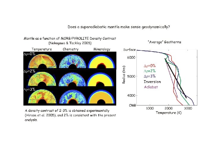
Is there any hope of (at least) an inversion consensus? Cammarano et al. ‘ 05: mantle is superadiabatic (if it’s pyrolite) Lyon Group: Mattern et al. ‘ 05 revisited by Matas et al. (pers. comm. ‘ 06) Khan et al. 08: travel time inversion, super-adiabatic non-pyrolitic; upper/lower mantle Mg/Si=1. 05 -1. 20

Is there a 660 layer? posterior prior

Mundane Conclusion The EM inversion results suggest a relatively homogeneous, superadiabatic mantle of chondritic composition More generally terrestrial inversions yield low Mg/Si (1. 05 -1. 2) and low bulk Ca. O and Al 2 O 3

Mars What is sort of known: Composition from a set of “Martian” meteorites (e. g. , Mc. Sween ’ 94) Core, but only a paleo-magnetic field (e. g. , Weiss et al. ‘ 02)

What is not known well at all: Thermal structure, core size and state from forward models that assume the SNC mantle composition and sensitive to crustal thickness What is known well: 4 Scalars (Yoder et al. ‘ 03) Mean mass and moment of inertia (distribution of mass) Second degree tidal Love number (squishyness ~ f(m. S, KS, r)) Tidal dissipation (inelasticity ~ g(m. S, qlocal))

Martian Mantle Composition

Martian Mantle Mineralogy No significant perovskite transition

Core Radius and Density

Areotherms and the Frozen Core Dilemma After Stewart & Schmidt ‘ 06

Martian Conclusions The Martian mantle is Fe-rich relative to Earth, but significantly less so than inferred from the SNC meteorites (Dreibus & Wanke ’ 85) The hot areotherm and large core radius preclude a Mgperovskite phase transition in the lower mantle (bad news for super-plumes? Not really) The martian core is far above its liquidus

“This is not the end, this is not even the beginning of the end, perhaps it is the end of the beginning. ” –- Winston Churchill Free energy minimization provides the basis for a general physical model that permits joint inversion of a priori unrelated geophysical data sets (seismic, gravity, electromagnetic)

Martian Temperature Distributions Prior Posterior

Seismic Velocities and Thermodynamic Consistency Sobolev & Babeyko ‘ 94 r no KS no m. S no Connolly & Kerrick ‘ 02 yes no Stixrude & Lithgow-Bertelloni ‘ 05 yes yes Does it really matter? Probably not, phase relations are most sensitive to integration constants and low-order derivatives, seismic velocities are most sensitive to highorder derivatives. Non-thermodynamic issues: anelasticity, aggregate modulii

Core Radius and CMB Temperature
")
Martian Inversion Resolution (T at 1200 km)

Trade-offs
 inversion (model 3)")
Mantle Conductivity Profile Olsen (’ 99) inversion (model 3)

Resolution and Stability
")
Phase equilibrium doesn't just provide parameters, but also an equation of state (Eo. S) that is essential to close the governing equations of geodynamic models. But what variables? Environment/Intensiv e System/Extensive Thermal T (diathermal) s (adiabatic) Mechanical P (inviscid) v (isochoric) Chemical m (mobile) m (inert) Homogeneous systems => common Eo. S choices: Khorzhinskii, k(P, T, m) Gibbs, g(P, T, m) Helmholtz, a(v, T, m) enthalpy, h(P, s, m) internal energy, u(v, s, m) u(s, v, m) is the only Eo. S for a heterogeneous system
? Discontinuous")
Putting g into geodynamics: What is the geodynamic equation of state (Eo. S)? Discontinuous reactions are singularities-> State changes, but the state function does not-> the Stefan problem
? Discontinuous")
Putting g into geodynamics: What is the geodynamic equation of state (Eo. S)? Discontinuous reactions are singularities-> State changes, but the state function does not-> the Stefan problem
? Discontinuous")
Putting g into geodynamics: What is the geodynamic equation of state (Eo. S)? Discontinuous reactions are singularities-> State changes, but the state function does not-> the Stefan problem
 We need h(s, P), we")
Optimization of exotic free energy functions: example h(s, P) We need h(s, P), we have g(T, P)…

Phase Diagrams: What, How, and, Maybe, Why by J. A. D. Connolly, ETH Phase diagram principles and nomenclature (Hillert 1986, Connolly 1990) Linearized solution of the phase equilibrium problem (Perple_X, Connolly 2009) Phase diagram applications in geophysics (Khan et al. 2006)
 We need h(s, P), we")
Optimization of exotic free energy functions: example h(s, P) We need h(s, P), we have g(T, P)… A hidden virtue of linearization: Discretization of h(T, P) for individual phases yields h(s, P) for the system, likewise u(T, P) yields u(s, v).

What does a calculated s-v phase diagram look like?
 into geodynamic models? *Mechanical work associated with the")
How do we put u(s, v) into geodynamic models? *Mechanical work associated with the Post-Perovskite transition is 5 times its Latent heat effect.

Computational Cycle

Look-up Tables Instead of Direct Calculation
, or any f(P, T) equation of")
A morsel of wisdom? Don’t put g(P, T), or any f(P, T) equation of state, into geodynamics Use u(s, v), it is easier than g and eliminates 1 st order phase transformations and thereby the Stefan problem

Forward Geodynamic Modelling: Subduction Zone Decarbonation Closed system models suggest carbonates in slab lithologies remain stable beyond sub-arc depths (Kerrick & Connolly, 1998, 2001 a, b). Would infiltration-driven decarbonation alter this conclusion?

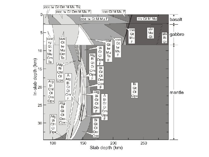

Slab fluid composition and production

Slab Properties Is infiltration decarbonation important? No. Taras Gerya is probably right!

Mapping Strategy

Free Energy Minimization by Linear Programming and Applications to Geophysical Inversion for Composition and Temperature Free Energy Minimization – a method for predicting thermodynamic (elastic) properties of rocks as a function of environmental variables (typically pressure and temperature) ®A forward model for rock properties: Geodynamic and Inversion calculations. ®A robust and efficient method. ®Some thoughts about cultural differences and data ®Two inversions for planetary composition and temperature

Optimize what when? And an Unexpected Virtue of the Linearized Solution Thermodynamics provides stability criterion (i. e. , an extremal function) for any choice of variables among the conjugate pairs P-V, T-S, m-n G(P, T, n) – inviscid, known temperature A(V, T, n) – known strain rate, temperature H(P, S, n) – inviscid, known heat flux U(S, V, n) – known strain rate and heat flux G(P, T, n) –> A, H, U as a f(P, T, n) Stefan Problem

Some thoughts about cultural differences and data Geophysics/Mineral physics • Limited data, lots of theory • Individual minerals and phase transitions • “A good experiment ****s any computation” D. Yuen, 2005 Pro: Amenable to simple parameterization for geodynamic models Con: Ignores strong autocorrelation of thermodynamic parameters Petrology • Lots of data, little theory • Global average Pro: Objectivity, single mega-parameter Con: Difficult to: assess uncertainty; separate first and second order affects; modify without access to primary data D” and the Fe-Mg-Al Post-perovskite transition
 into geodynamic models? The energy (aka temperature) equation")
How do we put u(s, v) into geodynamic models? The energy (aka temperature) equation as an example
?")
Putting g into geodynamics: What is the geodynamic equation of state (Eo. S)?
?")
Putting g into geodynamics: What is the geodynamic equation of state (Eo. S)?
?")
Putting g into geodynamics: What is the geodynamic equation of state (Eo. S)?

Linking Mineral Physics to Geophysics Mineral Physics: Mineral Properties Geophysics: Earth Properties

Linking Mineral Physics and Geophysics Petrology: Rock Properties Mineral Physics: Mineral Properties Geophysics: Earth Properties

The Non-Linear Phase Equilibrium Problem The stable state of a system minimizes its Gibbs Energy (G)
- Slides: 112