Thickness of Skull Hao Chai Dereck Shen Skull

Thickness of Skull Hao Chai Dereck Shen

Skull dataset � 138 skulls from 10 regions �Thickness was measured at 219 locations on each skull �Other variables in dataset: �Age of person (at time of death) �Sex of person �Dimensions of the skull (length/width/height)

Goals of the study �To determine what factors affect the thickness of the skull. If such effects exist, where on the skull do we see it? �Hannah is particularly interested in: (1) Sex effect (2) Climate effect (warm/cold)

Challenges/issues �Unbalanced data �Correlation structure �Multiple comparisons using Bonferroni correction

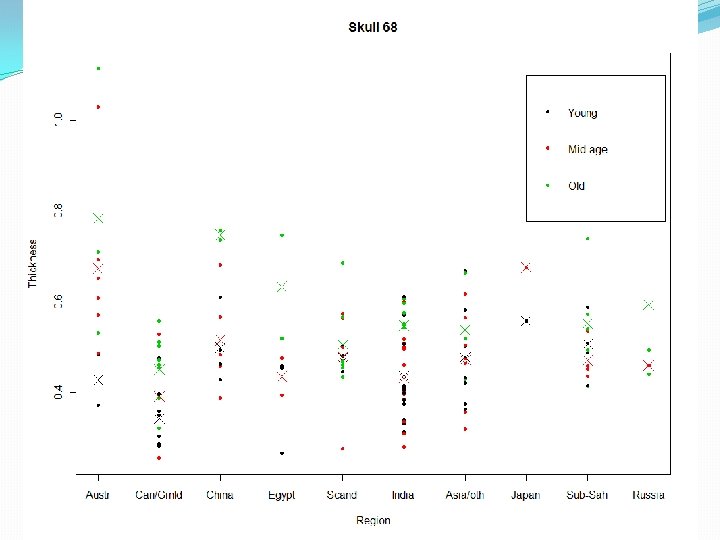
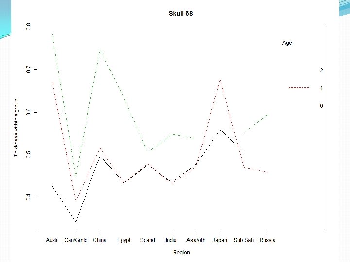
Changes to the dataset �Turned Age into a categorical variable: �Young (30 or younger) �Mid-age (between 30 and 45) �Old (45 or older) �Added a Climate factor derived from the regions: �Warm (Australia, Egypt, etc. ) �Cold (Scandinavia, Northern Russia, etc. ) �China (can’t be classified as either warm or cold)

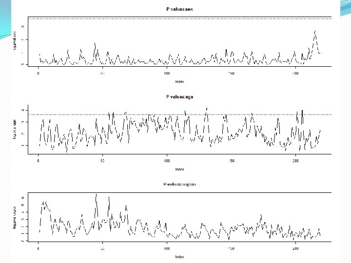
Classical analysis: Model 1 �At each location, we fitted an additive model with the following variables: �Three factors: Sex, Age, Region �Three covariates: Length/Width/Height of skull �Obtained the p-value of each factor using the Anova() function from ‘car’ package �Determine significance by comparing p-value to the Bonferroni-adjusted threshold: . 05/219

Anova() from ‘car’ �‘car’ stands for companion to applied regression; it’s a package written as a companion to a textbook �Anova() gives us the anova table with Type III tests �We don’t use the anova() function in the base package because it only provides us with Type I tests

Sample output with Anova()

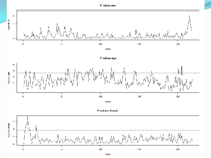
Classical analysis: Model 2 �Same as the first model, the only change is we replace the Region factor with the Climate factor

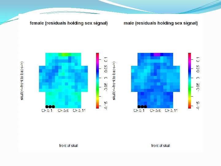
Results �Sex is not significant at any location �Age is significant at certain locations �Region is significant at certain locations �The number of locations where Climate is significant is fewer than that of Region, which suggests loss of information when we replace Region with Climate

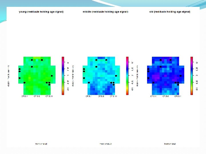
Using pixel plots to show age effect �At each location, fit the previous additive model without the Age factor �The residuals from the above model now hold the age signal �Using the pixel plot function from ‘spastat’ package, we can plot the average of the residuals at each location on a 2 -D map of the skull �We do this for each of the three age groups

Next step �Use permutation test to test for the effects