Theory of Probability Statistics for Business and Economics

Theory of Probability Statistics for Business and Economics Chap 4 -1

Randomness n n The term randomness suggests unpredictability A simple example of randomness is the tossing of a coin. The outcome is uncertain; it can either be an observed head (H) or an observed tail (T). Because the outcome of the toss cannot be predicted for sure, we say it displays randomness. Statistics for Business and Economics Chap 4 -2

Uncertainty n At some time or another, everyone will experience uncertainty. For example, you are approaching the traffic signals and the light changes from green to amber. You have to decide whether you can make it trough the intersection or not. You may be uncertain as to what the correct decision should be. Statistics for Business and Economics Chap 4 -3

Probability n The concept of probability is used to quantify this measure of doubt. If you believe that you have a 0. 99 probability of getting across the intersection, you have made a clear statement about your doubt. The probability statement provides a great deal of information, much more than statements such as “Maybe I can make it across” or “I should make it across” Statistics for Business and Economics Chap 4 -4

Important Definitions n n Random Experiment – a process leading to an uncertain outcome Basic Outcome – a possible outcome of a random experiment Sample Space – the collection of all possible outcomes of a random experiment Event – any subset of basic outcomes from the sample space Statistics for Business and Economics Chap 4 -5

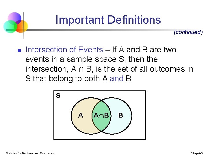
Important Definitions (continued) n Intersection of Events – If A and B are two events in a sample space S, then the intersection, A ∩ B, is the set of all outcomes in S that belong to both A and B S A Statistics for Business and Economics A B B Chap 4 -6

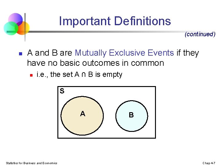
Important Definitions (continued) n A and B are Mutually Exclusive Events if they have no basic outcomes in common n i. e. , the set A ∩ B is empty S A Statistics for Business and Economics B Chap 4 -7

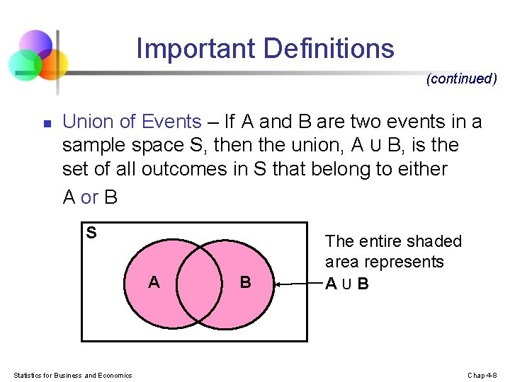
Important Definitions (continued) n Union of Events – If A and B are two events in a sample space S, then the union, A U B, is the set of all outcomes in S that belong to either A or B S A Statistics for Business and Economics B The entire shaded area represents AUB Chap 4 -8

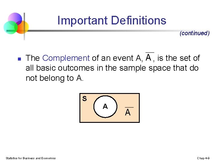
Important Definitions (continued) n The Complement of an event A, , is the set of all basic outcomes in the sample space that do not belong to A. S Statistics for Business and Economics A Chap 4 -9

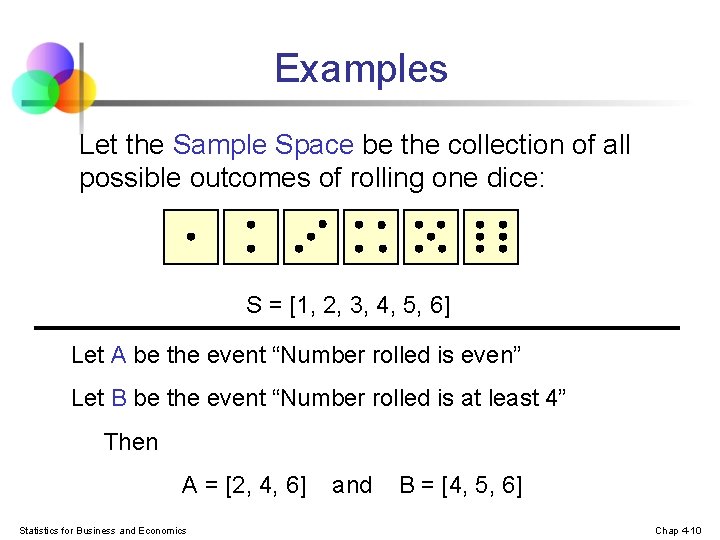
Examples Let the Sample Space be the collection of all possible outcomes of rolling one dice: S = [1, 2, 3, 4, 5, 6] Let A be the event “Number rolled is even” Let B be the event “Number rolled is at least 4” Then A = [2, 4, 6] Statistics for Business and Economics and B = [4, 5, 6] Chap 4 -10

Examples (continued) S = [1, 2, 3, 4, 5, 6] A = [2, 4, 6] B = [4, 5, 6] Complements: Intersections: Unions: Statistics for Business and Economics Chap 4 -11

Examples (continued) S = [1, 2, 3, 4, 5, 6] n B = [4, 5, 6] Mutually exclusive: n A and B are not mutually exclusive n n A = [2, 4, 6] The outcomes 4 and 6 are common to both Collectively exhaustive: n A and B are not collectively exhaustive n A U B does not contain 1 or 3 Statistics for Business and Economics Chap 4 -12

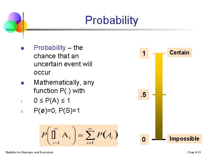
Probability n n i. ii. Probability – the chance that an uncertain event will occur Mathematically, any function P(. ) with 0 ≤ P(A) ≤ 1 P(ø)=0, P(S)=1 1 . 5 0 Statistics for Business and Economics Certain Impossible Chap 4 -13

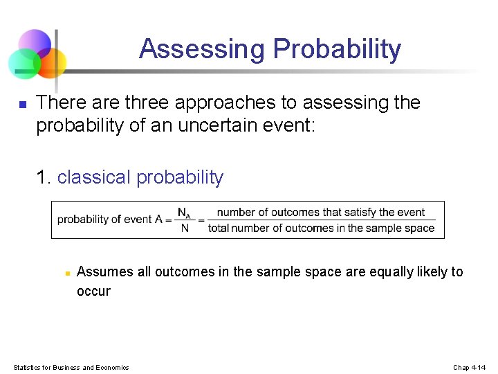
Assessing Probability n There are three approaches to assessing the probability of an uncertain event: 1. classical probability n Assumes all outcomes in the sample space are equally likely to occur Statistics for Business and Economics Chap 4 -14

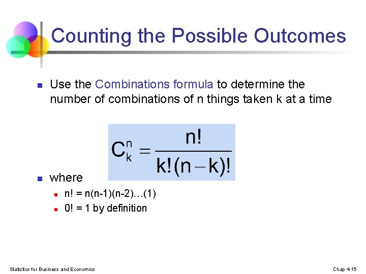
Counting the Possible Outcomes n n Use the Combinations formula to determine the number of combinations of n things taken k at a time where n n n! = n(n-1)(n-2)…(1) 0! = 1 by definition Statistics for Business and Economics Chap 4 -15

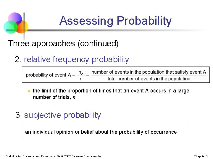
Assessing Probability Three approaches (continued) 2. relative frequency probability n the limit of the proportion of times that an event A occurs in a large number of trials, n 3. subjective probability an individual opinion or belief about the probability of occurrence Statistics for Business and Economics, 6 e © 2007 Pearson Education, Inc. Chap 4 -16

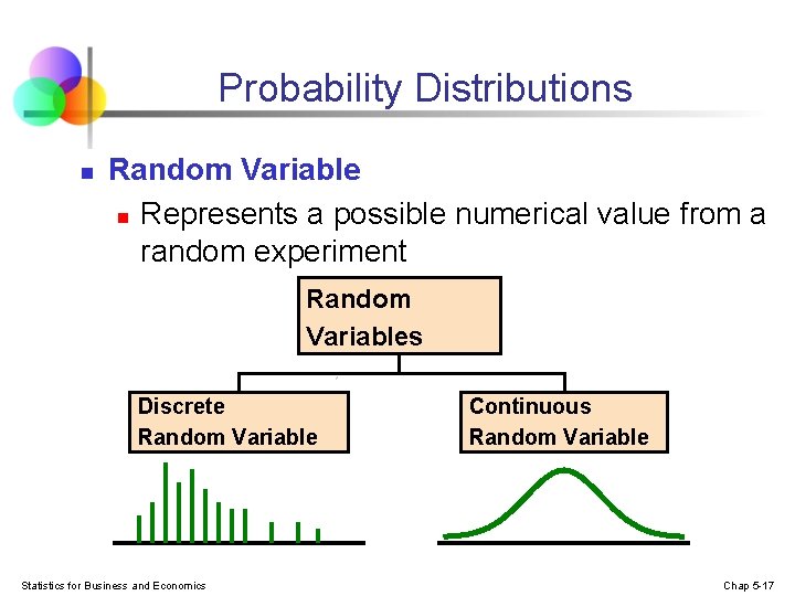
Probability Distributions n Random Variable n Represents a possible numerical value from a random experiment Random Variables Discrete Random Variable Statistics for Business and Economics Continuous Random Variable Chap 5 -17

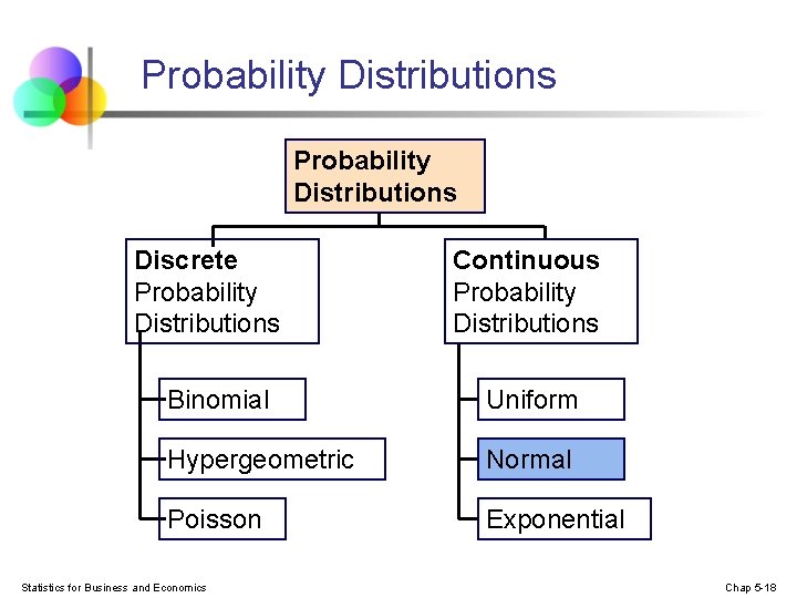
Probability Distributions Discrete Probability Distributions Continuous Probability Distributions Binomial Uniform Hypergeometric Normal Poisson Exponential Statistics for Business and Economics Chap 5 -18

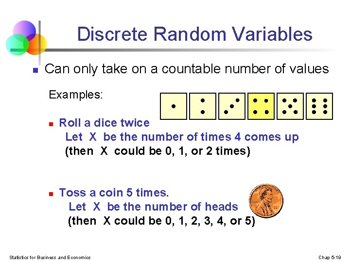
Discrete Random Variables n Can only take on a countable number of values Examples: n n Roll a dice twice Let X be the number of times 4 comes up (then X could be 0, 1, or 2 times) Toss a coin 5 times. Let X be the number of heads (then X could be 0, 1, 2, 3, 4, or 5) Statistics for Business and Economics Chap 5 -19

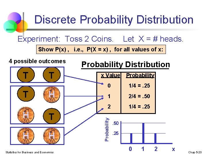
Discrete Probability Distribution Experiment: Toss 2 Coins. Let X = # heads. Show P(x) , i. e. , P(X = x) , for all values of x: T T H H T H Statistics for Business and Economics Probability Distribution x Value Probability 0 1/4 =. 25 1 2/4 =. 50 2 1/4 =. 25 Probability 4 possible outcomes . 50. 25 0 1 2 x Chap 5 -20

The Normal Distribution ‘Bell Shaped’ n Symmetrical f(x) n Mean, Median and Mode are Equal Location is determined by the mean, μ n Spread is determined by the standard deviation, σ The random variable has an infinite theoretical range: + to Statistics for Business and Economics σ μ x Mean = Median = Mode Chap 6 -21

The Normal Distribution (continued) n n The normal distribution closely approximates the probability distributions of a wide range of random variables Distributions of sample means approach a normal distribution given a “large” sample size Computations of probabilities are direct and elegant The normal probability distribution has led to good business decisions for a number of applications Statistics for Business and Economics Chap 6 -22

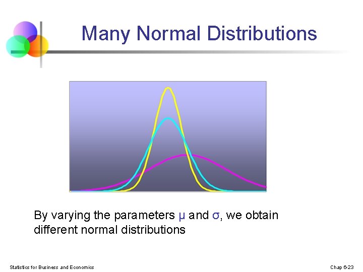
Many Normal Distributions By varying the parameters μ and σ, we obtain different normal distributions Statistics for Business and Economics Chap 6 -23

The Normal Distribution Shape f(x) Changing μ shifts the distribution left or right. σ μ Changing σ increases or decreases the spread. x Given the mean μ and variance σ we define the normal distribution using the notation Statistics for Business and Economics Chap 6 -24

The Normal Probability Density Function n The formula for the normal probability density function is Where e = the mathematical constant approximated by 2. 71828 π = the mathematical constant approximated by 3. 14159 μ = the population mean σ = the population standard deviation x = any value of the continuous variable, < x < Statistics for Business and Economics Chap 6 -25

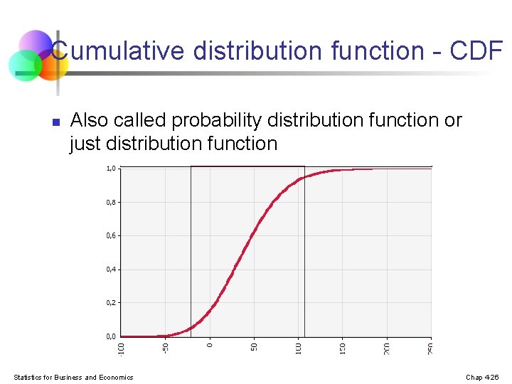
Cumulative distribution function - CDF n Also called probability distribution function or just distribution function Statistics for Business and Economics Chap 4 -26

Cumulative Probability Function n n The cumulative probability function, denoted F(x 0), shows the probability that X is less than or equal to x 0 In other words, Statistics for Business and Economics Chap 5 -27

Cumulative Normal Distribution n For a normal random variable X with mean μ and variance σ2 , i. e. , X~N(μ, σ2), the cumulative distribution function is f(x) 0 Statistics for Business and Economics x 0 x Chap 6 -28

CDF vs. pdf n n n Cumulative distribution function is an integral of probability density function Probability density function is a derivation of cumulative distribution function. CDF is defined only for values of a random variable X that are less than a certain value (x). CDF represents the surface under the probability density function. Statistics for Business and Economics Chap 4 -29

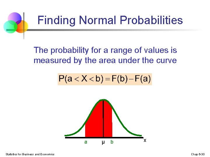
Finding Normal Probabilities The probability for a range of values is measured by the area under the curve a Statistics for Business and Economics μ b x Chap 6 -30

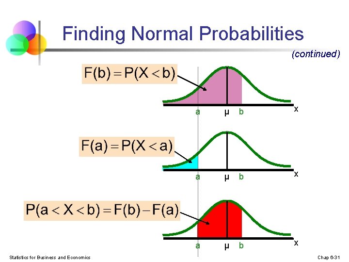
Finding Normal Probabilities (continued) Statistics for Business and Economics a μ b x Chap 6 -31

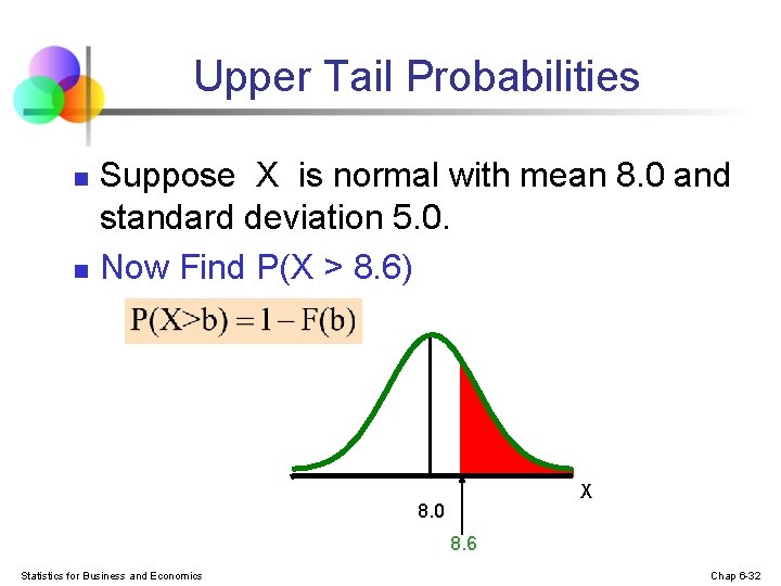
Upper Tail Probabilities n n Suppose X is normal with mean 8. 0 and standard deviation 5. 0. Now Find P(X > 8. 6) X 8. 0 8. 6 Statistics for Business and Economics Chap 6 -32

The Standardized Normal n Any normal distribution (with any mean and variance combination) can be transformed into the standardized normal distribution (Z), with mean 0 and variance 1 f(Z) 1 0 n Z Need to transform X units into Z units by subtracting the mean of X and dividing by its standard deviation Statistics for Business and Economics Chap 6 -33

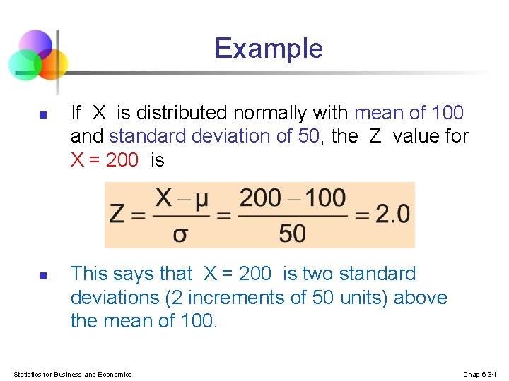
Example n n If X is distributed normally with mean of 100 and standard deviation of 50, the Z value for X = 200 is This says that X = 200 is two standard deviations (2 increments of 50 units) above the mean of 100. Statistics for Business and Economics Chap 6 -34

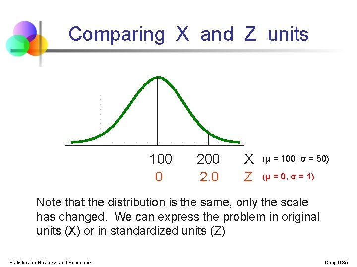
Comparing X and Z units 100 0 200 2. 0 X Z (μ = 100, σ = 50) (μ = 0, σ = 1) Note that the distribution is the same, only the scale has changed. We can express the problem in original units (X) or in standardized units (Z) Statistics for Business and Economics Chap 6 -35

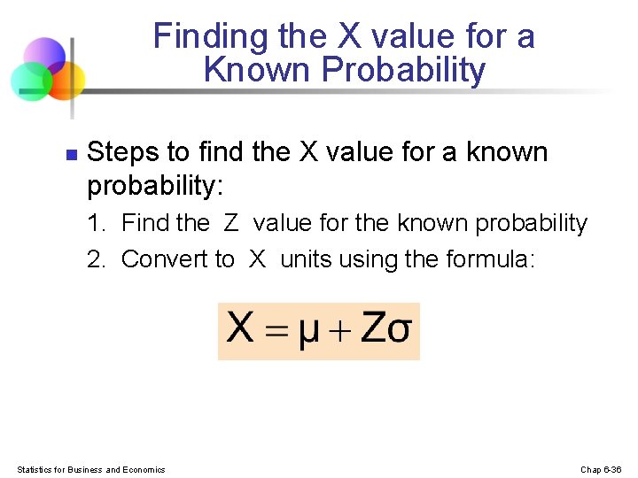
Finding the X value for a Known Probability n Steps to find the X value for a known probability: 1. Find the Z value for the known probability 2. Convert to X units using the formula: Statistics for Business and Economics Chap 6 -36

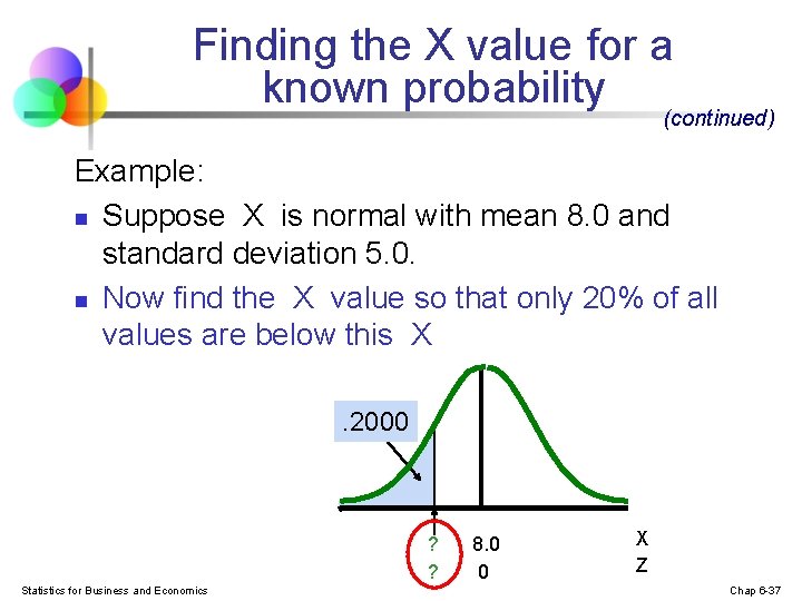
Finding the X value for a known probability (continued) Example: n Suppose X is normal with mean 8. 0 and standard deviation 5. 0. n Now find the X value so that only 20% of all values are below this X. 2000 ? ? Statistics for Business and Economics 8. 0 0 X Z Chap 6 -37

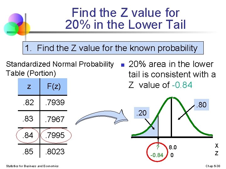
Find the Z value for 20% in the Lower Tail 1. Find the Z value for the known probability Standardized Normal Probability Table (Portion) z F(z) . 82 . 7939 . 83 . 7967 . 84 . 7995 . 8023 Statistics for Business and Economics n 20% area in the lower tail is consistent with a Z value of -0. 84. 80 . 20 ? 8. 0 -0. 84 0 X Z Chap 6 -38

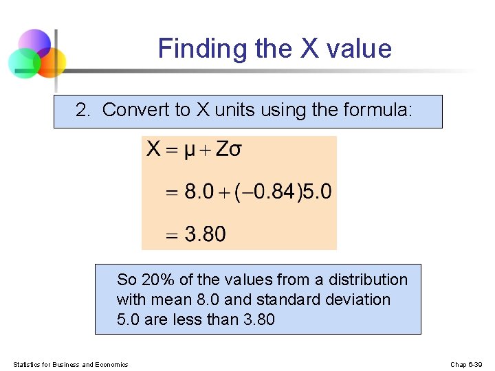
Finding the X value 2. Convert to X units using the formula: So 20% of the values from a distribution with mean 8. 0 and standard deviation 5. 0 are less than 3. 80 Statistics for Business and Economics Chap 6 -39

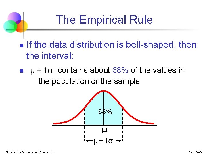
The Empirical Rule n n If the data distribution is bell-shaped, then the interval: contains about 68% of the values in the population or the sample 68% Statistics for Business and Economics Chap 3 -40

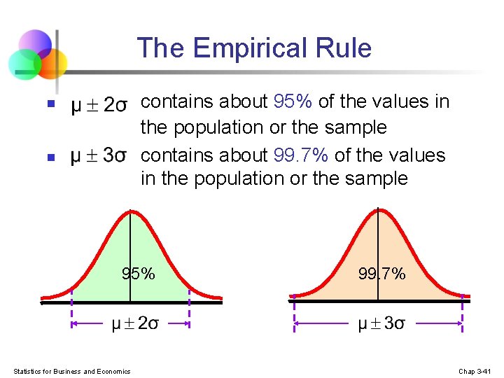
The Empirical Rule contains about 95% of the values in the population or the sample contains about 99. 7% of the values in the population or the sample n n 95% Statistics for Business and Economics 99. 7% Chap 3 -41

Next topic n Point and interval estimate Thank you! Have a nice day!