THEORETICAL PROBABILITY DISTRIBUTION THEORETICAL PROBABILITY DISTRIBUTION Introduction Types

THEORETICAL PROBABILITY DISTRIBUTION

THEORETICAL PROBABILITY DISTRIBUTION • Introduction • Types • Binomial Distribution • Poisson Distribution • Normal Distribution • Examples

PROBABILITY DISTRIBUTION • Theoretical probability distribution of a variable may be – Theoretical listing of outcomes and probabilities which can be obtained from a mathematical model representing some phenomenon of interest – Observed probability distributions • Based on actual observations and experimentation • Obtained by grouping data • Help understanding properly the nature of data

THEORETICAL PROBABILITY DISTRIBUTION • It is possible to deduce mathematically what the frequency distribution of certain population should be • These distributions based on previous experience or theoretical considerations are theoretical probability distributions • Example: Tossing of coin 100 times – Expected outcome 50% each – Actual out come may be 40% and 60% – Experiment carried out large number of times average gets close to 50% head and 50% tail

THEORETICAL PROBABILITY DISTRIBUTION • Random variable is a numerical quantity whose value is determined by the outcome of a random experiment • Probability distribution for a discrete random variable is mutually exclusive listing of all possible numerical outcomes for that random variable

RANDOM VARIABLE • The mathematical rule (or function) that assigns a given numerical value to each possible outcome of an experiment in the sample space of interest

RANDOM VARIABLES • Discrete random variable (X): If set of values defined by it over the sample space is finite – Probability function P(X) is ‘probability mass function’ and distribution ‘discrete probability distribution’ • Continuous random variables (X): If it can assume any value in an interval – Probability function P(X) is ‘probability density function’ and distribution ‘continuous probability distribution’

WHY? • Act as substitutes for actual distributions when latter are costly to obtain or cannot be obtained at all • Useful in making predictions on the basis of limited information or theoretical considerations • Form a basis for more advanced statistical methods – ‘fit’ between observed distributions and certain theoretical distributions is an assumption of many statistical procedures

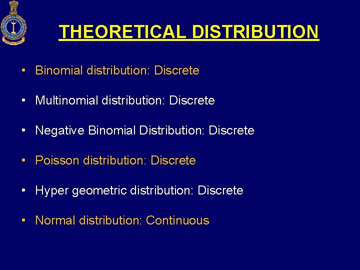
THEORETICAL DISTRIBUTION • Binomial distribution: Discrete • Multinomial distribution: Discrete • Negative Binomial Distribution: Discrete • Poisson distribution: Discrete • Hyper geometric distribution: Discrete • Normal distribution: Continuous

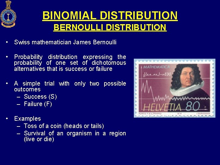
BINOMIAL DISTRIBUTION BERNOULLI DISTRIBUTION • Swiss mathematician James Bernoulli • Probability distribution expressing the probability of one set of dichotomous alternatives that is success or failure • A simple trial with only two possible outcomes – Success (S) – Failure (F) • Examples – Toss of a coin (heads or tails) – Survival of an organism in a region (live or die) Jacob Bernoulli (1654 -1705)

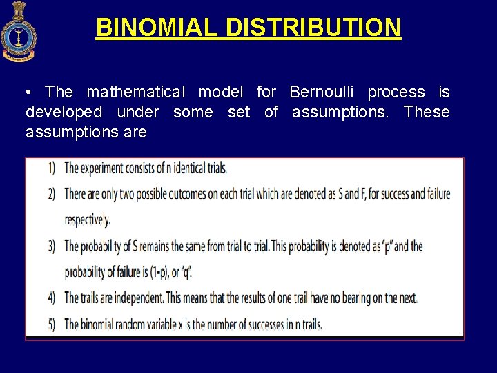
BINOMIAL DISTRIBUTION • The mathematical model for Bernoulli process is developed under some set of assumptions. These assumptions are Example: dart game

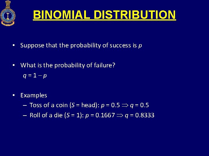
BINOMIAL DISTRIBUTION • Suppose that the probability of success is p • What is the probability of failure? q=1–p • Examples – Toss of a coin (S = head): p = 0. 5 q = 0. 5 – Roll of a die (S = 1): p = 0. 1667 q = 0. 8333

BINOMIAL DISTRIBUTION • Imagine that a trial is repeated n times • Examples – A coin is tossed 5 times – A die is rolled 25 times • p remains constant from trial to trial and that the trials are statistically independent of each other

BINOMIAL DISTRIBUTION • What is the probability of obtaining x successes in n trials? • Trials result in a series of success and failures, FFSFFFFSFSFSSFFFFFSF… Then the probability of x successes in that order is P(x) = q q p q = px q n – x

BINOMIAL DISTRIBUTION • However, if order is not important, then P ( x) = where n! x!(n – x)! in n trials n! x!(n – x)! px q n – x is the number of ways to obtain x successes

BINOMIAL DISTRIBUTION • The binomial distribution with parameters n and p is the discrete probability distribution of the number of successes in a sequence of n independent yes/no experiments, each of which yields success with probability p • The binomial distribution is frequently used to model the number of successes in a sample of size n drawn with replacement from a population of size N

BINOMIAL DISTRIBUTION • If the sampling is carried out without replacement, the draws are not independent and so the resulting distribution is not a binomial one. • For N much larger than n, the binomial distribution is a good approximation, and widely used • In general, if the random variable X follows the binomial distribution with parameters n and p, we write X ~ B(n, p)

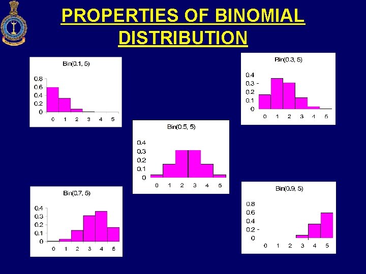
PROPERTIES OF BINOMIAL DISTRIBUTION • The shape and location of binomial distribution changes as p changes for a given n or as n changes for a given p. As p increase for a fixed n, the binomial distribution shits to right

PROPERTIES OF BINOMIAL DISTRIBUTION

PROPERTIES OF BINOMIAL DISTRIBUTION • When p and q are equal the distribution is symmetrical. When p and q are not equal distribution is skew. If p <1/2, distribution is positively skewed • The mode of Binomial distribution is equal to the value of x which has the largest probability – For example if n = 6 and p = 0. 3 the mode is equal to 2. For n = 6 and p = 0. 9 the mode is equal to 6 • The mean of Binomial distribution is np and SD (npq)1/2 • If n is large and if neither p nor q is too close to zero, the binomial distribution can be closely approximated by a normal distribution

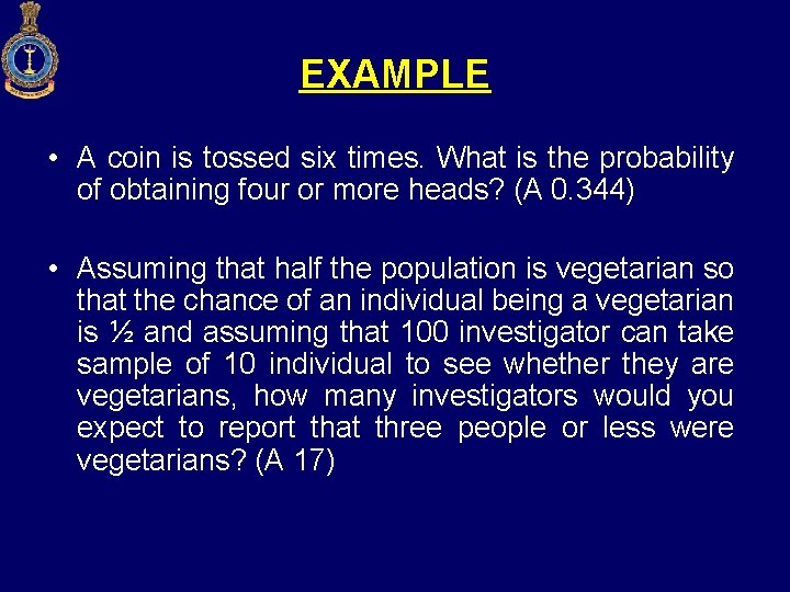
EXAMPLE • A coin is tossed six times. What is the probability of obtaining four or more heads? (A 0. 344) • Assuming that half the population is vegetarian so that the chance of an individual being a vegetarian is ½ and assuming that 100 investigator can take sample of 10 individual to see whether they are vegetarians, how many investigators would you expect to report that three people or less were vegetarians? (A 17)

FITTING BINOMIAL DISTRIBUTION • Procedure – Determine p and q, when p and q are equal the distribution is symmetrical. When p and q are not equal distribution is skew. If p <1/2, distribution is positively skewed – Expand the binomial (p+q)n when two coins are tossed n=2, when four coins are tossed n=4 – Multiply each term of the expanded binomial by N (the total frequency), in order to obtain the expected frequency in each category

FITTING BINOMIAL DISTRIBUTION – 8 coins are tossed at a time 256 times. Number of heads observed at each throw is recorded and the results are given below. Find the expected frequencies. What are theoretical values of mean and standard deviation? Calculate also the mean and SD of the observed frequencies?

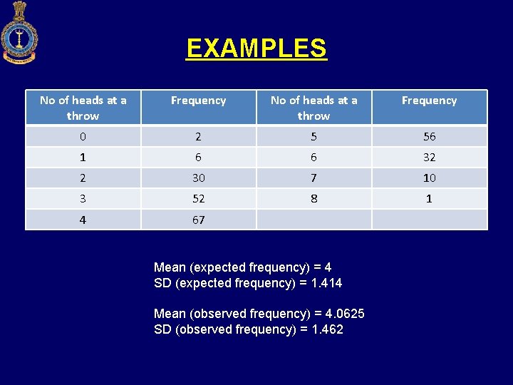
EXAMPLES No of heads at a throw Frequency 0 2 5 56 1 6 6 32 2 30 7 10 3 52 8 1 4 67 Mean (expected frequency) = 4 SD (expected frequency) = 1. 414 Mean (observed frequency) = 4. 0625 SD (observed frequency) = 1. 462

POISSON DISTRIBUTION • Discrete distribution • Distribution is expected in cases where the chance of any individual event being a success is small • Used to describe the behavior of rare events • Law of improbable events Simeon D. Poisson (17811840)

THE POISSON DISTRIBUTION • When there is a large number of trials, but a small probability of success, binomial calculation becomes impractical Example: 64 deaths in 20 years from thousands of soldiers • The mean number of successes from n trials is µ = np Simeon D. Poisson (17811840)

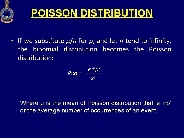
POISSON DISTRIBUTION • If we substitute µ/n for p, and let n tend to infinity, the binomial distribution becomes the Poisson distribution: P(x) = e -µµx x! Where µ is the mean of Poisson distribution that is ‘np’ or the average number of occurrences of an event

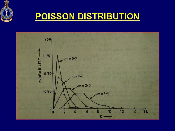
POISSON DISTRIBUTION • Poisson distribution is with single parameter µ, as µ increases the distribution shifts to the right • Poisson distribution is applied where random rare events in space or time are expected to occur • Deviation from Poisson distribution may indicate some degree of non-randomness in the events under study • Investigation of cause may be of interest • All Poisson prob distributions are skewed to the right

POISSON DISTRIBUTION

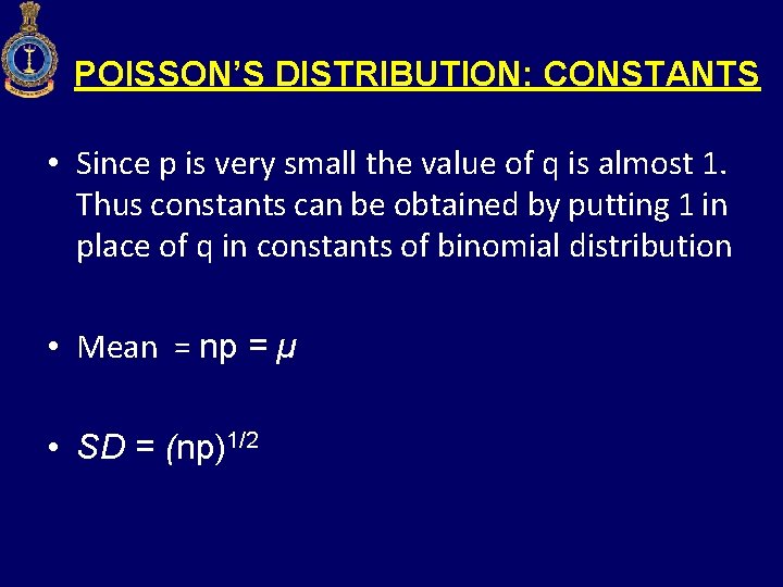
POISSON’S DISTRIBUTION: CONSTANTS • Since p is very small the value of q is almost 1. Thus constants can be obtained by putting 1 in place of q in constants of binomial distribution • Mean = np = µ • SD = (np)1/2

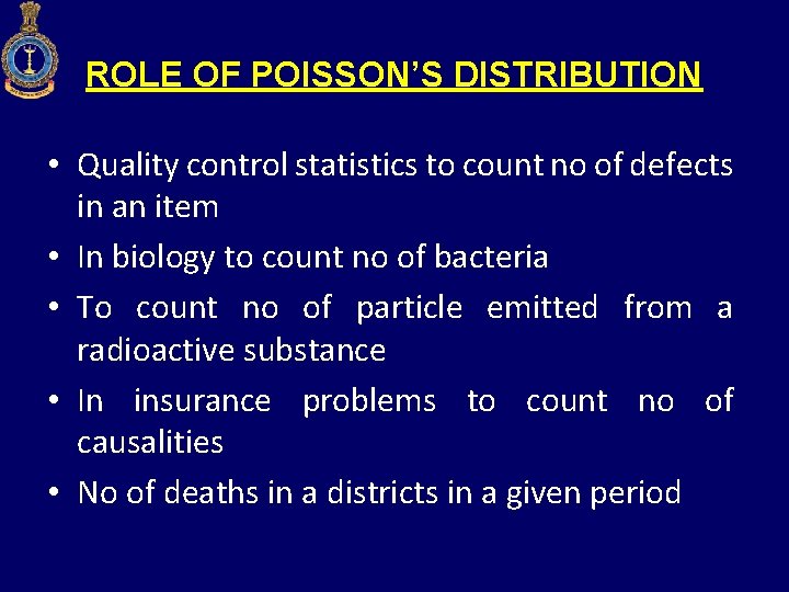
ROLE OF POISSON’S DISTRIBUTION • Quality control statistics to count no of defects in an item • In biology to count no of bacteria • To count no of particle emitted from a radioactive substance • In insurance problems to count no of causalities • No of deaths in a districts in a given period

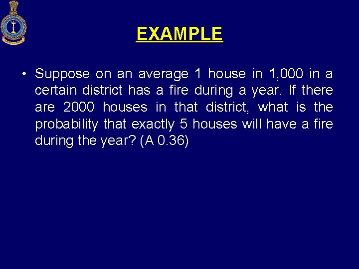
EXAMPLE • Suppose on an average 1 house in 1, 000 in a certain district has a fire during a year. If there are 2000 houses in that district, what is the probability that exactly 5 houses will have a fire during the year? (A 0. 36)

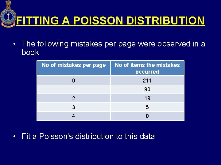
FITTING A POISSON DISTRIBUTION • The following mistakes per page were observed in a book No of mistakes per page No of items the mistakes occurred 0 211 1 90 2 19 3 5 4 0 • Fit a Poisson's distribution to this data

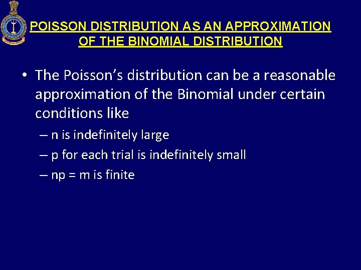
POISSON DISTRIBUTION AS AN APPROXIMATION OF THE BINOMIAL DISTRIBUTION • The Poisson’s distribution can be a reasonable approximation of the Binomial under certain conditions like – n is indefinitely large – p for each trial is indefinitely small – np = m is finite

NORMAL DISTRIBUTION • Binomial and Poisson distribution for discrete random variable • Mathematical distribution for continuously varying variable is required • Normal distribution • Most useful theoretical distribution for continuous variable

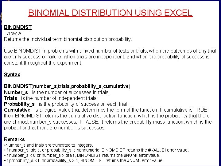
BINOMIAL DISTRIBUTION USING EXCEL BINOMDIST how All Returns the individual term binomial distribution probability. S Use BINOMDIST in problems with a fixed number of tests or trials, when the outcomes of any trial are only success or failure, when trials are independent, and when the probability of success is constant throughout the experiment. Syntax BINOMDIST(number_s, trials, probability_s, cumulative) Number_s is the number of successes in trials. Trials is the number of independent trials. Probability_s is the probability of success on each trial. Cumulative is a logical value that determines the form of the function. If cumulative is TRUE, then BINOMDIST returns the cumulative distribution function, which is the probability that there at most number_s successes; if FALSE, it returns the probability mass function, which is the probability that there are number_s successes. Remarks • Number_s and trials are truncated to integers. • If number_s, trials, or probability_s is nonnumeric, BINOMDIST returns the #VALUE! error value. • If number_s < 0 or number_s > trials, BINOMDIST returns the #NUM! error value. • If probability_s < 0 or probability_s > 1, BINOMDIST returns the #NUM! error value.

Check Also !! CRITBINOM(trials, probability_s, alpha) • Trials is the number of Bernoulli trials. • Probability_s is the probability of a success on each trial. • Alpha is the criterion value. Returns the smallest value for which the cumulative binomial distribution is greater than or equal to a criterion value. Use this function for quality assurance applications. For example, use CRITBINOM to determine the greatest number of defective parts that are allowed to come off an assembly line run without rejecting the entire lot.

POISSON DISTRIBUTION USING EXCEL Returns the Poisson distribution. A common application of the Poisson distribution is predicting the number of events over a specific time, such as the number of cars arriving at a toll plaza in 1 minute. Syntax POISSON(x, mean, cumulative) X is the number of events. Mean is the expected numeric value. Cumulative is a logical value that determines the form of the probability distribution returned. If cumulative is TRUE, POISSON returns the cumulative Poisson probability that the number of random events occurring will be between zero and x inclusive; if FALSE, it returns the Poisson probability mass function that the number of events occurring will be exactly x.

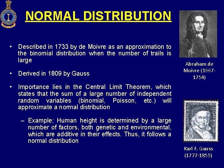
NORMAL DISTRIBUTION • Described in 1733 by de Moivre as an approximation to the binomial distribution when the number of trails is large • Derived in 1809 by Gauss Abraham de Moivre (16671754) • Importance lies in the Central Limit Theorem, which states that the sum of a large number of independent random variables (binomial, Poisson, etc. ) will approximate a normal distribution – Example: Human height is determined by a large number of factors, both genetic and environmental, which are additive in their effects. Thus, it follows a normal distribution Karl F. Gauss (1777 -1855)

NORMAL (GAUSSIAN) DISTRIBUTION • It is an approximation to binomial distribution • Whether or not p is equal to q, n becomes large • Tails stretch infinitely in both directions

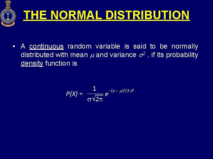
THE NORMAL DISTRIBUTION • A continuous random variable is said to be normally distributed with mean and variance 2 , if its probability density function is 1 (x )2/2 2 P(X) = e 2

NORMAL (GAUSSIAN) DISTRIBUTION • A single normal curve exists for any combination of , – these are the parameters of the distribution and define it completely • The normal distribution can have different shapes depending on different values of , , but there is one and only one normal distribution for any given pair of values for and

NORMAL DISTRIBUTION • Normal distribution limiting case of binomial distribution when N is too large and neither p nor q is very small • Normal distribution limiting case of Poisson distribution when mean is large • The mean of a normally distributed population lies at the centre of its normal curve • Two tails of the normal probability distribution extend indefinitely and never touch horizontal axis • Positive probability for continuous random variable

NORMAL DISTRIBUTION: PROPERTIES • For continuous variable • Curve is bell shaped and symmetrical appearance, mean and median coincide in • Normal distribution is defined by its , • Every normal distribution has its own , • The mean, median distribution are equal and mode of normal

NORMAL DISTRIBUTION: PROPERTIES • The area under the curve is 1 • Distribution denser in the center and less so in the trails • Trails never touch the axis, range is unlimited in both directions • Normal curve is unimodal, has only one mode

NORMAL DISTRIBUTION: PROPERTIES • The area under the normal curve is distributed as – Mean + 1 covers 68. 27% area, 34. 135 area on either side of the mean – Mean + 2 covers 95. 45% area – Mean + 3 covers 99. 73% area

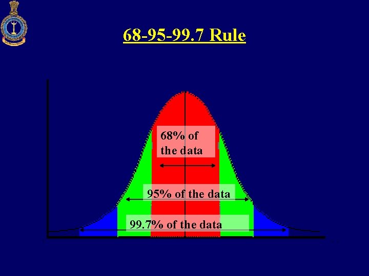
68 -95 -99. 7 Rule 68% of the data 95% of the data 99. 7% of the data

CONDITIONS FOR NORMALITY • The casual forces must be numerous and of approximately equal weight • The forces must be same over the universe from which observations are drawn (condition of homogeneity) • The forces affecting events must be independent of one another • The operation of the casual forces must be such that deviation above the population mean are balanced as to magnitude and number by deviations below the mean (conditions of symmetry)

AREA RELATIONSHIP § The area of the normal curve between § Mean Ordinate § Ordinate at various sigma distance from the mean (as percentage of the total area) 52

STANDARD NORMAL DISTRIBUTION

AREA UNDER NORMAL CURVE § How to convert Normal curve with mean x and standard deviation By performing § Change of scale from X to Z Scale § Change of origin σ § In original scale X – scale mean and standard deviation are µ & § In new scale Z-scale mean = 0 and SD = 1

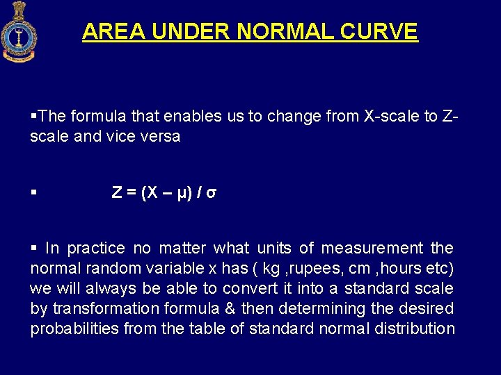
AREA UNDER NORMAL CURVE §The formula that enables us to change from X-scale to Zscale and vice versa § Z = (X – μ) / σ § In practice no matter what units of measurement the normal random variable x has ( kg , rupees, cm , hours etc) we will always be able to convert it into a standard scale by transformation formula & then determining the desired probabilities from the table of standard normal distribution

AREA UNDER NORMAL CURVE § The transformation from X to Z is termed as Ztransformation. § Given a value of X , the corresponding Z value tell us : § How far away § What direction X is from its mean in terms of its standard deviation σ Z = 1. 8 means that the value σ to the right of mean x of X is 1. 8

AREA UNDER NORMAL CURVE • Area under the curve , corresponding to a normal distribution equal to unity, regardless of particular number of observations involved • We thus have a Normal Distribution that is independent of • Number of observations • Mean • Standard deviation • This is known as UNIT NORMAL DISTRIBUTION OR STANDARD NORMAL DISTRIBUTION • It is applicable to any distribution that is normal regardless of mean, SD & No of Observations

RELATION BETWEEN THREE DISTRIBUTIONS § Binomial (large ‘n’ and small ‘p’) → Poisson Distribution § Poisson (large ‘m’) → Normal Distribution 58

NORMAL DISTRIBUTION EXAMPLE § Given is the mean height of soldiers as 68. 22 inches, with variance of 10. 8 inches. How many soldiers are expected to be above 72 inches out of strength of 1000? § Assuming distribution is normal, following values are given: X = 72; μ = 68. 22; σ2 = 10. 8

NORMAL DISTRIBUTION EXAMPLE § σ2 = 10. 8, so σ = 3. 286 § Hence, Z = (X – μ) / σ = 1. 16 § Note the value from the table for ‘Z’, which is 0. 3749 § Probability of 72 inches or more height is required, so area to its right is to be found § Area to the right of this value is: 0. 5000 – 0. 3749 = 0. 1251 which is the required probability

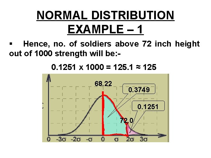
NORMAL DISTRIBUTION EXAMPLE – 1 § Hence, no. of soldiers above 72 inch height out of 1000 strength will be: 0. 1251 x 1000 = 125. 1 ≈ 125 68. 22 0. 3749 0. 1251 72. 0

NORMDIST USING EXCEL Returns the normal distribution for the specified mean and standard deviation. This function has a very wide range of applications in statistics, including hypothesis testing. Syntax NORMDIST(x, mean, standard_dev, cumulative) X is the value for which you want the distribution. Mean is the arithmetic mean of the distribution. Standard_dev is the standard deviation of the distribution. Cumulative is a logical value that determines the form of the function. If cumulative is TRUE, NORMDIST returns the cumulative distribution function; if FALSE, it returns the probability mass function. 62

NORMINV Returns the inverse of the normal cumulative distribution for the specified mean and standard deviation. Syntax NORMINV(probability, mean, standard_dev) Probability is a probability corresponding to the normal distribution. Mean is the arithmetic mean of the distribution. Standard_dev is the standard deviation of the distribution. BPKC : CLM (STATS) 63

NORMSDIST Returns the standard normal cumulative distribution function. The distribution has a mean of 0 (zero) and a standard deviation of one. Use this function in place of a table of standard normal curve areas. Syntax NORMSDIST(z) Z is the value for which you want the distribution. BPKC : CLM (STATS) 64

NORMSINV Returns the inverse of the standard normal cumulative distribution. The distribution has a mean of zero and a standard deviation of one. Syntax NORMSINV(probability) Probability is a probability corresponding to the normal distribution. Remarks • If probability is nonnumeric, NORMSINV returns the #VALUE! error value. • If probability < 0 or if probability > 1, NORMSINV returns the #NUM! error value. Given a value for probability, NORMSINV seeks that value z such that NORMSDIST(z) = probability. Thus, precision of NORMSINV depends on precision of NORMSDIST. NORMSINV uses an iterative search technique. If BPKC : CLM (STATS) the search has not converged after 100 iterations, the function returns the 65 #N/A error value.

? BPKC : CLM (STATS) 66