Theme 6 Linear regression 1 Introduction 2 The

Theme 6. Linear regression 1. Introduction. 2. The equation of the line. 3. The least squares criterion. 4. Graphical representation. 5. Standardized regression coefficients. 6. The coefficient of determination. 7. Introduction to multiple regression.

Introduction The establishment of a correlation between two variables is important, but this is considered a first step when predicting one variable from the other. (Or others, in the case of multiple regression; ie. , multiple predictors. ) Of course, if we know that the variable X is closely related to Y, this means that we can predict Y from X. We are now in the field of prediction. (Obviously if X is unrelated to Y, X does not serve as predictor of Y. ) Note: We will use the terms "regression" and "prediction" as almost synonymous. (The reason for the use of the term "regression" is old, and has remained as such. )

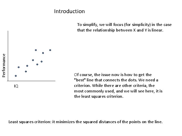
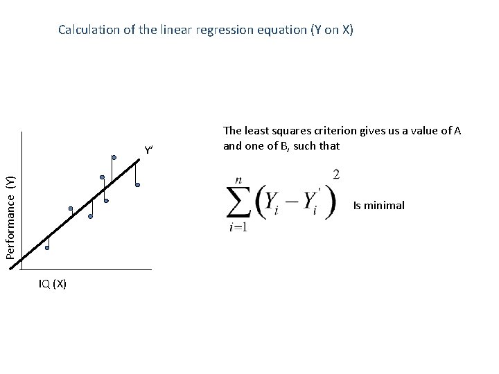
Introduction Performance To simplify, we will focus (for simplicity) in the case that the relationship between X and Y is linear. IQ Of course, the issue now is how to get the "best" line that connects the dots. We need a criterion. While there are other criteria, the most commonly used, and we will see here, it is the least squares criterion. Least squares criterion: it minimizes the squared distances of the points on the line.

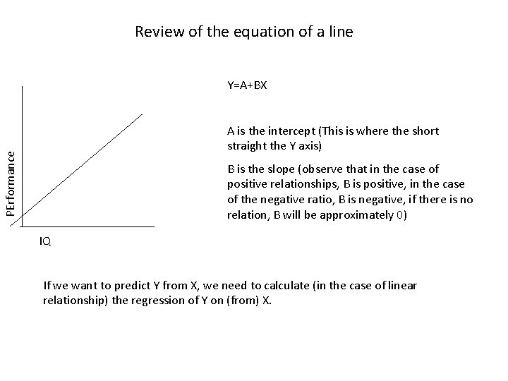
Review of the equation of a line Y=A+BX PErformance A is the intercept (This is where the short straight the Y axis) B is the slope (observe that in the case of positive relationships, B is positive, in the case of the negative ratio, B is negative, if there is no relation, B will be approximately 0) IQ If we want to predict Y from X, we need to calculate (in the case of linear relationship) the regression of Y on (from) X.

Calculation of the linear regression equation (Y on X) Performance (Y) Y’ The least squares criterion gives us a value of A and one of B, such that Is minimal IQ (X)

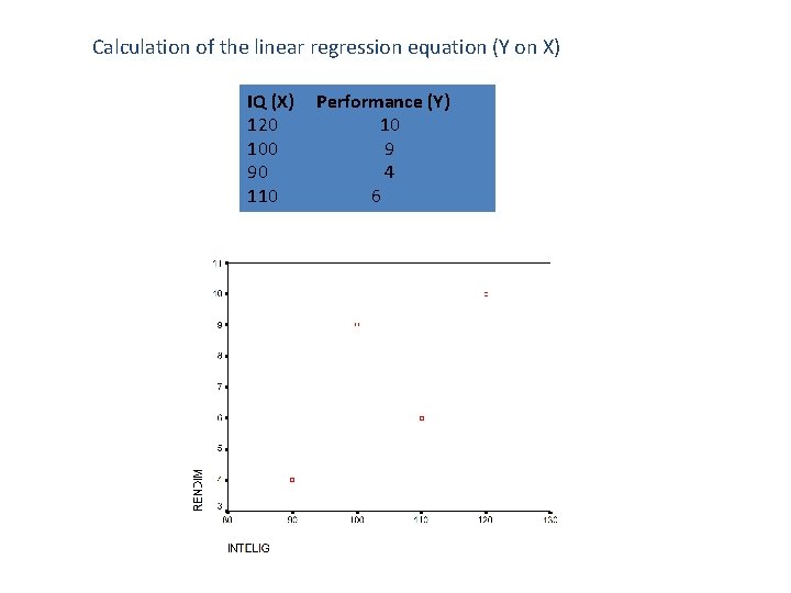
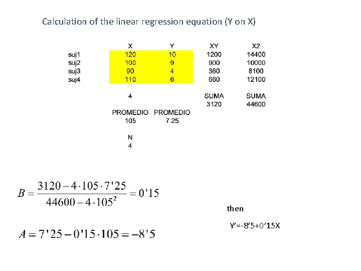
Calculation of the linear regression equation (Y on X) IQ (X) Performance (Y) 120 10 100 9 90 4 110 6

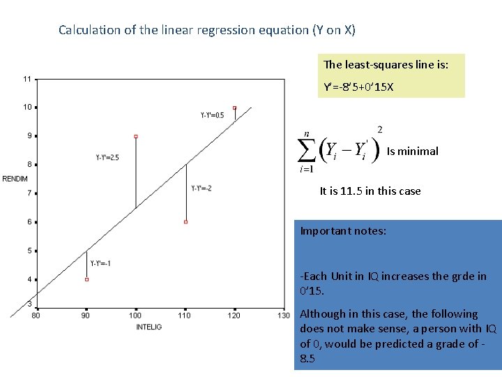
Calculation of the linear regression equation (Y on X) The least-squares line is: Y’=-8’ 5+0’ 15 X Is minimal It is 11. 5 in this case Important notes: -Each Unit in IQ increases the grde in 0’ 15. Although in this case, the following does not make sense, a person with IQ of 0, would be predicted a grade of 8. 5

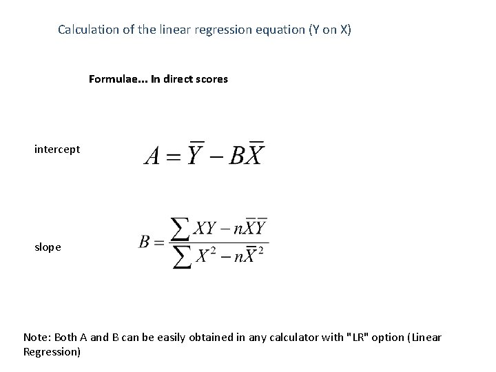
Calculation of the linear regression equation (Y on X) Formulae. . . In direct scores intercept slope Note: Both A and B can be easily obtained in any calculator with "LR" option (Linear Regression)

Calculation of the linear regression equation (Y on X) then Y’=-8’ 5+0’ 15 X

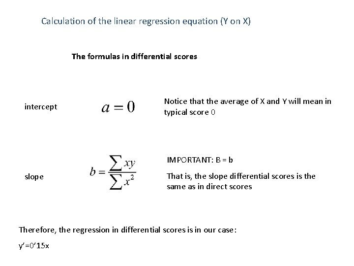
Calculation of the linear regression equation (Y on X) The formulas in differential scores intercept Notice that the average of X and Y will mean in typical score 0 IMPORTANT: B = b slope That is, the slope differential scores is the same as in direct scores Therefore, the regression in differential scores is in our case: y’=0’ 15 x

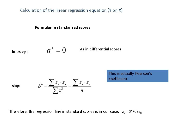
Calculation of the linear regression equation (Y on X) Formulas in standarized scores intercept As in differential scores This is actually Pearson’s coefficient slope Therefore, the regression line in standard scores is in our case: zy’ =0’ 703 zx

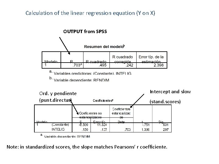
Calculation of the linear regression equation (Y on X) OUTPUT from SPSS Ord. y pendiente (punt. directas) Intercept and slow (stand. scores) Note: in standardized scores, the slope matches Pearsons’ r coefficiente.

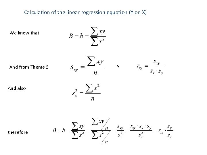
Calculation of the linear regression equation (Y on X) We know that And from Theme 5 And also therefore y

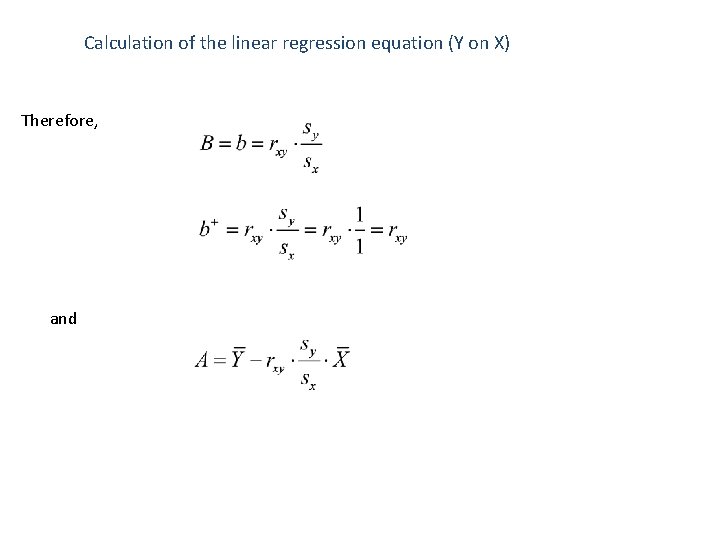
Calculation of the linear regression equation (Y on X) Therefore, and

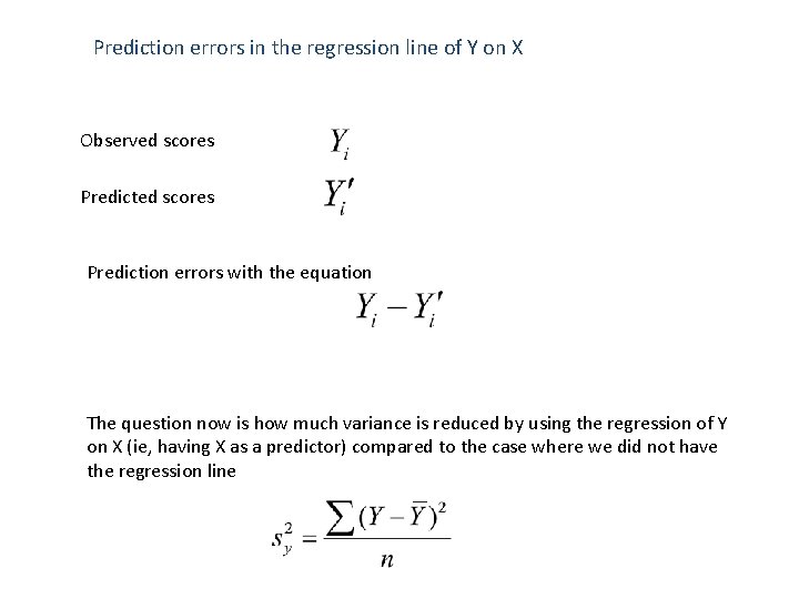
Prediction errors in the regression line of Y on X Observed scores Prediction errors with the equation The question now is how much variance is reduced by using the regression of Y on X (ie, having X as a predictor) compared to the case where we did not have the regression line

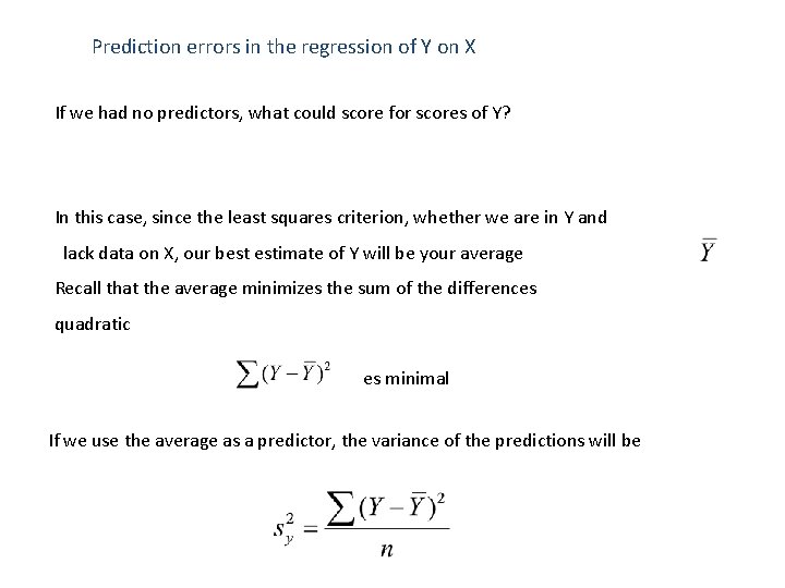
Prediction errors in the regression of Y on X If we had no predictors, what could score for scores of Y? In this case, since the least squares criterion, whether we are in Y and lack data on X, our best estimate of Y will be your average Recall that the average minimizes the sum of the differences quadratic es minimal If we use the average as a predictor, the variance of the predictions will be

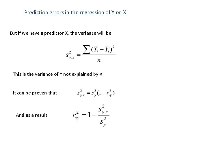
Prediction errors in the regression of Y on X But if we have a predictor X, the variance will be This is the variance of Y not explained by X It can be proven that And as a result

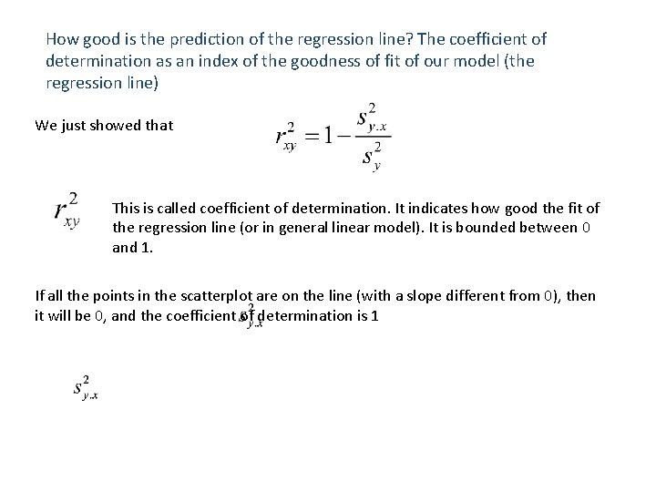
How good is the prediction of the regression line? The coefficient of determination as an index of the goodness of fit of our model (the regression line) We just showed that This is called coefficient of determination. It indicates how good the fit of the regression line (or in general linear model). It is bounded between 0 and 1. If all the points in the scatterplot are on the line (with a slope different from 0), then it will be 0, and the coefficient of determination is 1

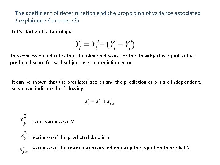
The coefficient of determination and the proportion of variance associated / explained / Common (2) Let's start with a tautology This expression indicates that the observed score for the ith subject is equal to the predicted score for said subject over a prediction error. It can be shown that the predicted scores and the prediction errors are independent, so we can indicate the following Total variance of Y Variance of the predicted data in Y Variance of the residuals (errors) when using the equation to predict Y

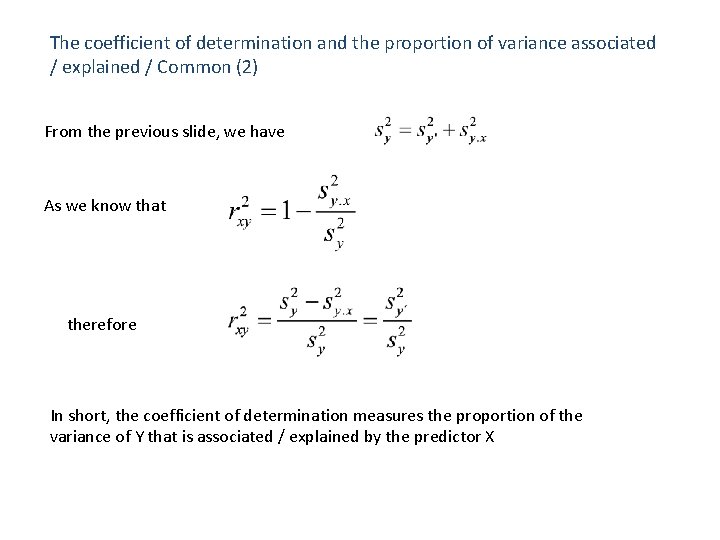
The coefficient of determination and the proportion of variance associated / explained / Common (2) From the previous slide, we have As we know that therefore In short, the coefficient of determination measures the proportion of the variance of Y that is associated / explained by the predictor X

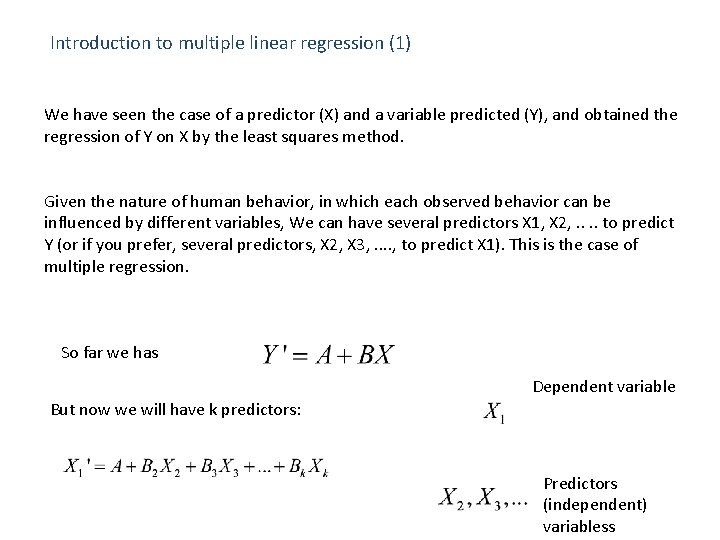
Introduction to multiple linear regression (1) We have seen the case of a predictor (X) and a variable predicted (Y), and obtained the regression of Y on X by the least squares method. Given the nature of human behavior, in which each observed behavior can be influenced by different variables, We can have several predictors X 1, X 2, . . to predict Y (or if you prefer, several predictors, X 2, X 3, . . , to predict X 1). This is the case of multiple regression. So far we has Dependent variable But now we will have k predictors: Predictors (independent) variabless

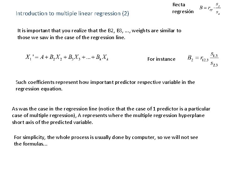
Introduction to multiple linear regression (2) Recta regresión It is important that you realize that the B 2, B 3, . . . , weights are similar to those we saw in the case of the regression line. For instance Such coefficients represent how important predictor respective variable in the regression equation. As was the case in the regression line (notice that the case of 1 predictor is a particular case of multiple regression), A represents where the multiple regression hyperplane short axis of the predicted variable. For simplicity, the whole process is usually done by computer, so we will not see the formulas. . .

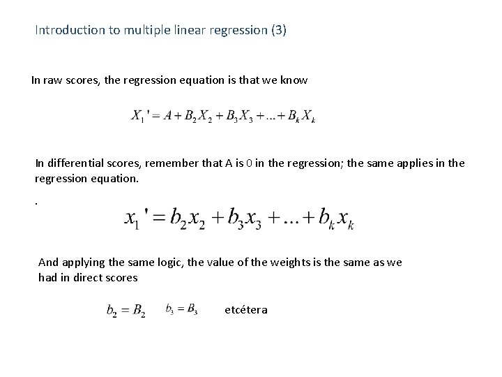
Introduction to multiple linear regression (3) In raw scores, the regression equation is that we know In differential scores, remember that A is 0 in the regression; the same applies in the regression equation. . And applying the same logic, the value of the weights is the same as we had in direct scores etcétera

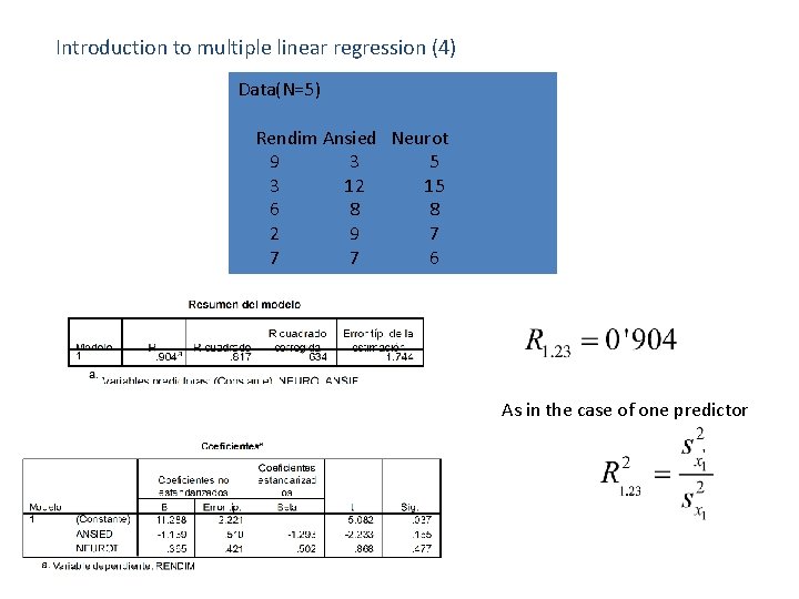
Introduction to multiple linear regression (4) Data(N=5) Rendim Ansied Neurot 9 3 5 3 12 15 6 8 8 2 9 7 7 7 6 As in the case of one predictor

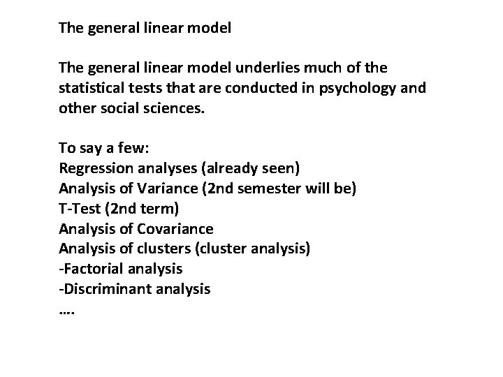
The general linear model underlies much of the statistical tests that are conducted in psychology and other social sciences. To say a few: Regression analyses (already seen) Analysis of Variance (2 nd semester will be) T-Test (2 nd term) Analysis of Covariance Analysis of clusters (cluster analysis) -Factorial analysis -Discriminant analysis ….

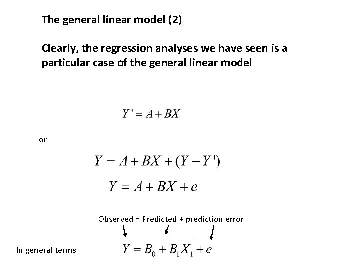
The general linear model (2) Clearly, the regression analyses we have seen is a particular case of the general linear model or Observed = Predicted + prediction error In general terms

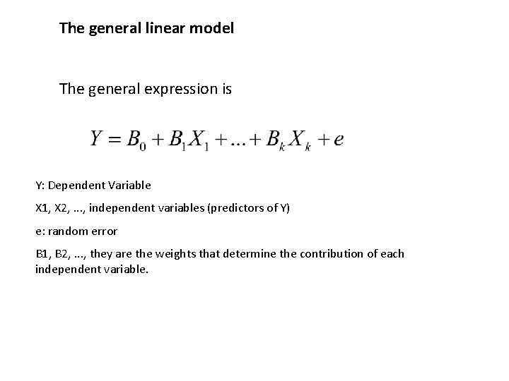
The general linear model The general expression is Y: Dependent Variable X 1, X 2, . . . , independent variables (predictors of Y) e: random error B 1, B 2, . . . , they are the weights that determine the contribution of each independent variable.