The Weighted Majority Algorithm How to do as

The Weighted Majority Algorithm How to do as well as the best algorithm.

Using “expert” advice Say we want to predict the stock market. • We solicit N “experts” for their advice. (Will the market go up or down? ) • We then want to use their advice somehow to make our prediction. E. g. , Can we do nearly as well as best in hindsight? [“expert” ´ someone with an opinion. Not necessarily someone who knows anything. ]

Simpler question • We have N “experts”. • One of these is perfect (never makes a mistake). We just don’t know which one. • Can we find a strategy that makes no more than lg(N) mistakes? Answer: sure. Just take majority vote over all experts that have been correct so far. ØEach mistake cuts # available by factor of 2. ØNote: this means ok for N to be very large. “halving algorithm”

Using “expert” advice But what if none is perfect? Can we do nearly as well as the best one in hindsight? Strategy #1: • Iterated halving algorithm. Same as before, but once we've crossed off all the experts, restart from the beginning. • Makes at most lg(N)[OPT+1] mistakes, where OPT is #mistakes of the best expert in hindsight. Seems wasteful. Constantly forgetting what we've “learned”. Can we do better?

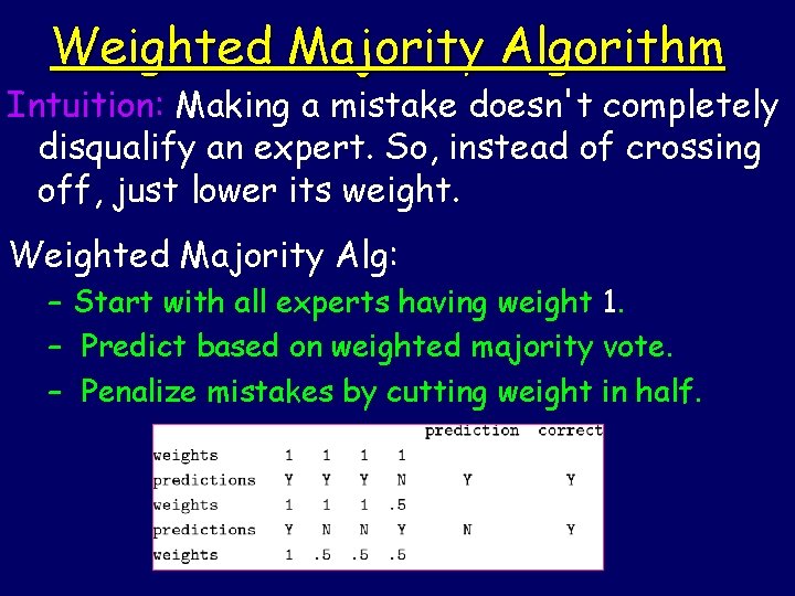
Weighted Majority Algorithm Intuition: Making a mistake doesn't completely disqualify an expert. So, instead of crossing off, just lower its weight. Weighted Majority Alg: – Start with all experts having weight 1. – Predict based on weighted majority vote. – Penalize mistakes by cutting weight in half.

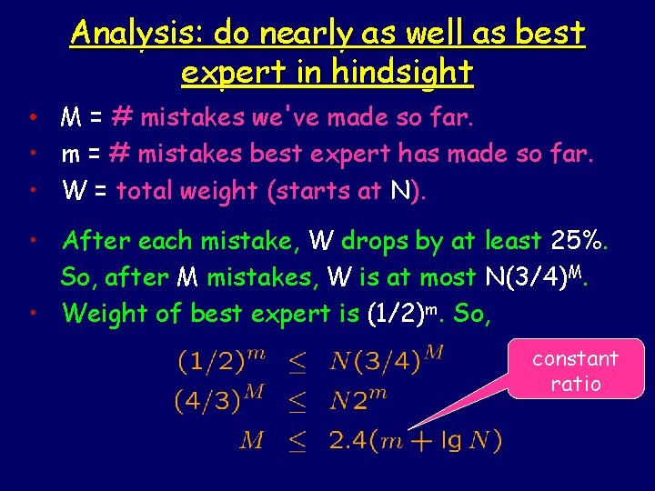
Analysis: do nearly as well as best expert in hindsight • M = # mistakes we've made so far. • m = # mistakes best expert has made so far. • W = total weight (starts at N). • After each mistake, W drops by at least 25%. So, after M mistakes, W is at most N(3/4)M. • Weight of best expert is (1/2)m. So, constant ratio

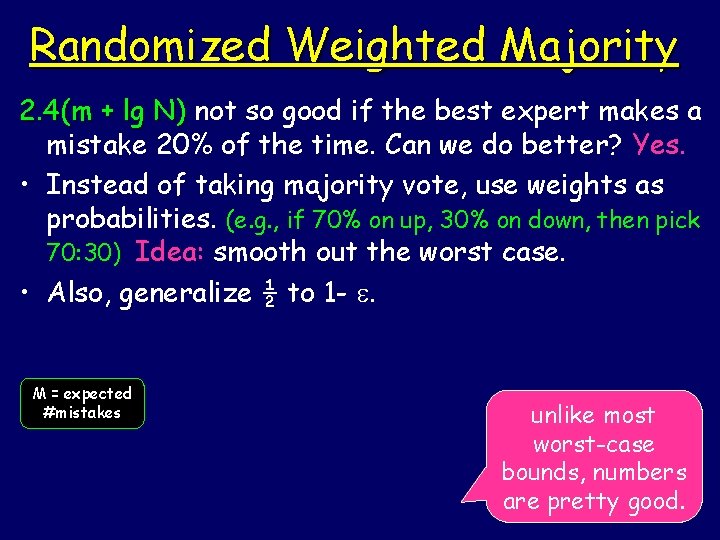
Randomized Weighted Majority 2. 4(m + lg N) not so good if the best expert makes a mistake 20% of the time. Can we do better? Yes. • Instead of taking majority vote, use weights as probabilities. (e. g. , if 70% on up, 30% on down, then pick 70: 30) Idea: smooth out the worst case. • Also, generalize ½ to 1 - . M = expected #mistakes unlike most worst-case bounds, numbers are pretty good.

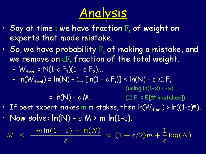
Analysis • Say at time t we have fraction Ft of weight on experts that made mistake. • So, we have probability Ft of making a mistake, and we remove an Ft fraction of the total weight. – Wfinal = N(1 - F 1)(1 - F 2). . . – ln(Wfinal) = ln(N) + t [ln(1 - Ft)] < ln(N) - t Ft (using ln(1 -x) < -x) = ln(N) - M. ( Ft = E[# mistakes]) • If best expert makes m mistakes, then ln(Wfinal) > ln((1 - )m). • Now solve: ln(N) - M > m ln(1 - ).

Summarizing • E[# mistakes] < (1+ )m + -1 log(N). • If set =(log(N)/m)1/2 to balance the two terms out (or use guess-and-double), get bound of E[mistakes] = m+2(mlog N)1/2 • Since m < T, this is at most m + 2(Tlog N)1/2. • So, competitive ratio = 1.

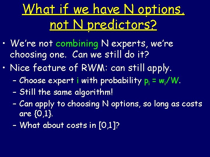
What if we have N options, not N predictors? • We’re not combining N experts, we’re choosing one. Can we still do it? • Nice feature of RWM: can still apply. – Choose expert i with probability pi = wi/W. – Still the same algorithm! – Can apply to choosing N options, so long as costs are {0, 1}. – What about costs in [0, 1]?

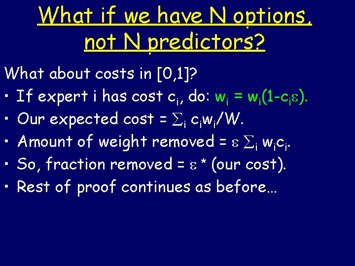
What if we have N options, not N predictors? What about costs in [0, 1]? • If expert i has cost ci, do: wi = wi(1 -ci ). • Our expected cost = i ciwi/W. • Amount of weight removed = i wici. • So, fraction removed = * (our cost). • Rest of proof continues as before…

Stop 2: Game Theory

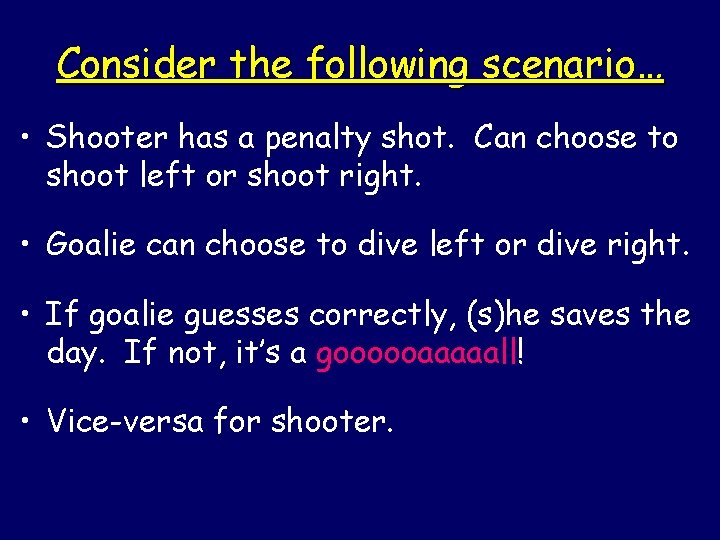
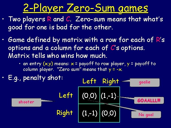
Consider the following scenario… • Shooter has a penalty shot. Can choose to shoot left or shoot right. • Goalie can choose to dive left or dive right. • If goalie guesses correctly, (s)he saves the day. If not, it’s a goooooaaaaall! • Vice-versa for shooter.

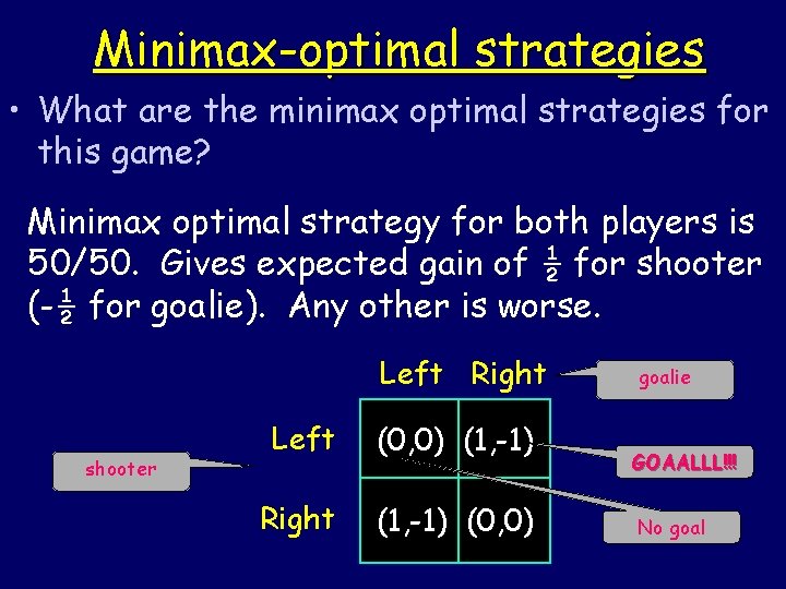
2 -Player Zero-Sum games • Two players R and C. Zero-sum means that what’s good for one is bad for the other. • Game defined by matrix with a row for each of R’s options and a column for each of C’s options. Matrix tells who wins how much. • an entry (x, y) means: x = payoff to row player, y = payoff to column player. “Zero sum” means that y = -x. • E. g. , penalty shot: shooter Left Right Left (0, 0) (1, -1) Right (1, -1) (0, 0) goalie GOAALLL!!! No goal

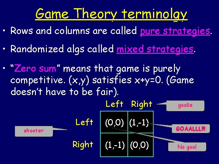
Game Theory terminolgy • Rows and columns are called pure strategies. • Randomized algs called mixed strategies. • “Zero sum” means that game is purely competitive. (x, y) satisfies x+y=0. (Game doesn’t have to be fair). Left Right shooter Left (0, 0) (1, -1) Right (1, -1) (0, 0) goalie GOAALLL!!! No goal

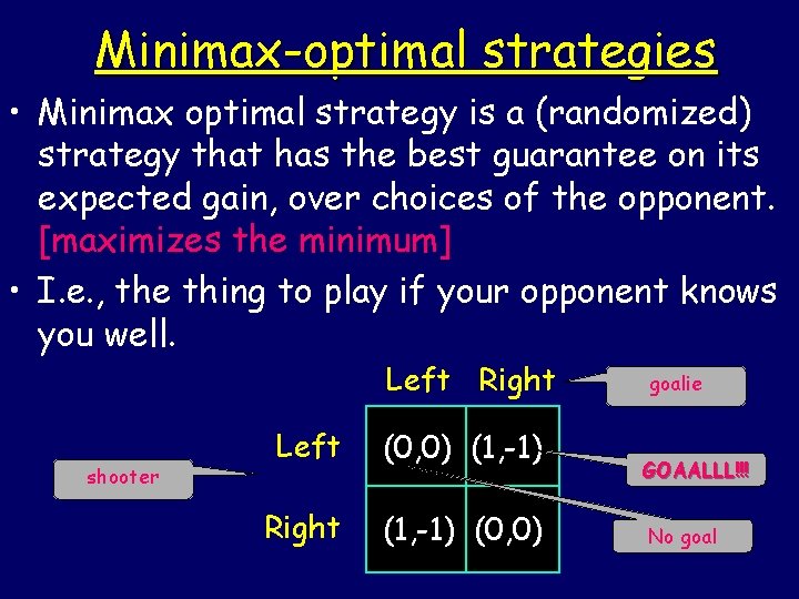
Minimax-optimal strategies • Minimax optimal strategy is a (randomized) strategy that has the best guarantee on its expected gain, over choices of the opponent. [maximizes the minimum] • I. e. , the thing to play if your opponent knows you well. Left Right shooter Left (0, 0) (1, -1) Right (1, -1) (0, 0) goalie GOAALLL!!! No goal

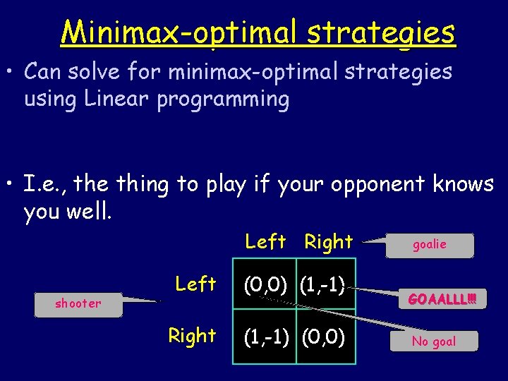
Minimax-optimal strategies • Can solve for minimax-optimal strategies using Linear programming • I. e. , the thing to play if your opponent knows you well. Left Right shooter Left (0, 0) (1, -1) Right (1, -1) (0, 0) goalie GOAALLL!!! No goal

Minimax-optimal strategies • What are the minimax optimal strategies for this game? Minimax optimal strategy for both players is 50/50. Gives expected gain of ½ for shooter (-½ for goalie). Any other is worse. Left Right shooter Left (0, 0) (1, -1) Right (1, -1) (0, 0) goalie GOAALLL!!! No goal

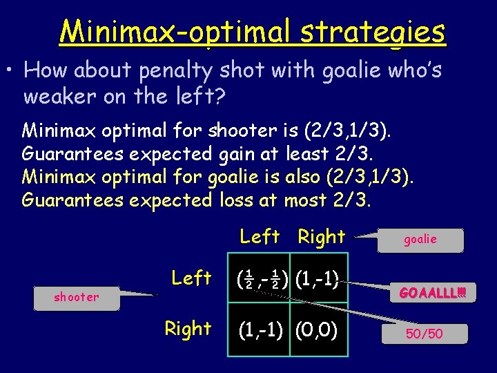
Minimax-optimal strategies • How about penalty shot with goalie who’s weaker on the left? Minimax optimal for shooter is (2/3, 1/3). Guarantees expected gain at least 2/3. Minimax optimal for goalie is also (2/3, 1/3). Guarantees expected loss at most 2/3. Left Right shooter Left (½, -½) (1, -1) Right (1, -1) (0, 0) goalie GOAALLL!!! 50/50

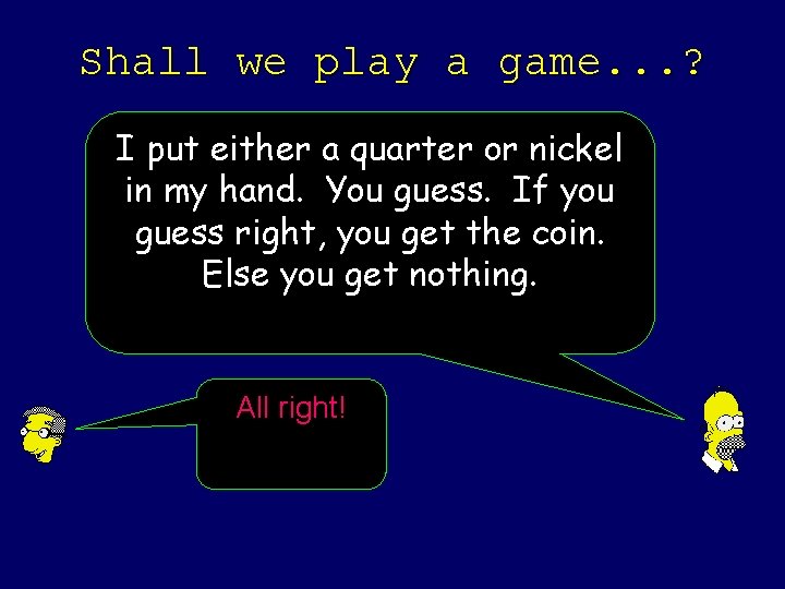
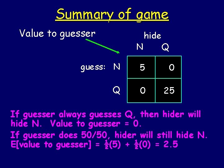
Shall we play a game. . . ? I put either a quarter or nickel in my hand. You guess. If you guess right, you get the coin. Else you get nothing. All right!

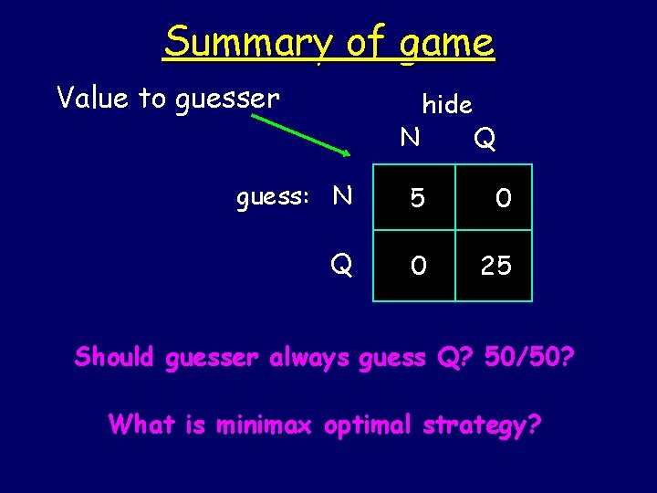
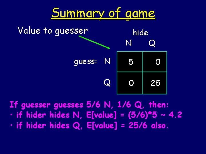
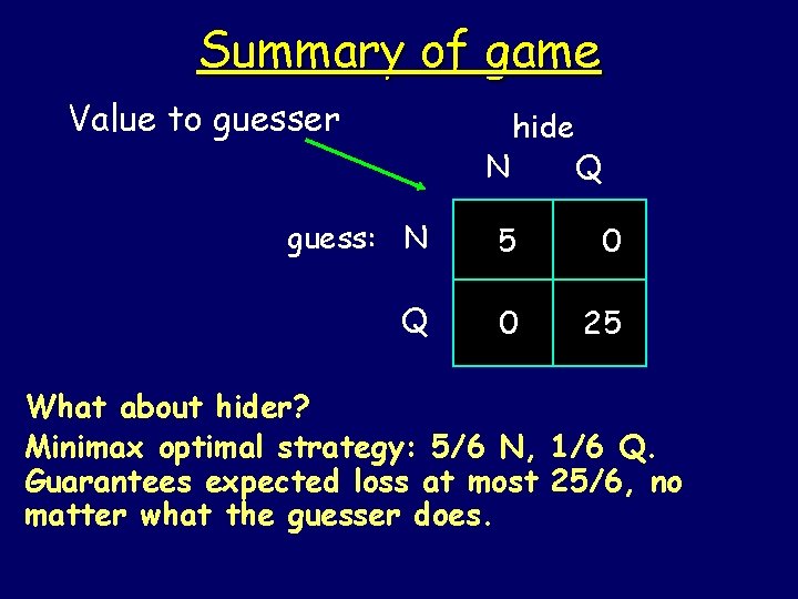
Summary of game Value to guesser N hide Q guess: N 5 0 Q 0 25 Should guesser always guess Q? 50/50? What is minimax optimal strategy?

Summary of game Value to guesser N hide Q guess: N 5 0 Q 0 25 If guesser always guesses Q, then hider will hide N. Value to guesser = 0. If guesser does 50/50, hider will still hide N. E[value to guesser] = ½(5) + ½(0) = 2. 5

Summary of game Value to guesser N hide Q guess: N 5 0 Q 0 25 If guesser guesses 5/6 N, 1/6 Q, then: • if hider hides N, E[value] = (5/6)*5 ~ 4. 2 • if hider hides Q, E[value] = 25/6 also.

Summary of game Value to guesser N hide Q guess: N 5 0 Q 0 25 What about hider? Minimax optimal strategy: 5/6 N, 1/6 Q. Guarantees expected loss at most 25/6, no matter what the guesser does.

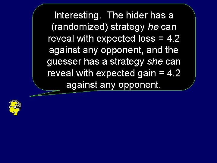
Interesting. The hider has a (randomized) strategy he can reveal with expected loss = 4. 2 against any opponent, and the guesser has a strategy she can reveal with expected gain = 4. 2 against any opponent.

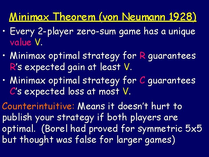
Minimax Theorem (von Neumann 1928) • Every 2 -player zero-sum game has a unique value V. • Minimax optimal strategy for R guarantees R’s expected gain at least V. • Minimax optimal strategy for C guarantees C’s expected loss at most V. Counterintuitive: Means it doesn’t hurt to publish your strategy if both players are optimal. (Borel had proved for symmetric 5 x 5 but thought was false for larger games)

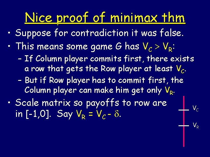
Nice proof of minimax thm • Suppose for contradiction it was false. • This means some game G has VC > VR: – If Column player commits first, there exists a row that gets the Row player at least VC. – But if Row player has to commit first, the Column player can make him get only VR. • Scale matrix so payoffs to row are in [-1, 0]. Say VR = VC - . VC VR

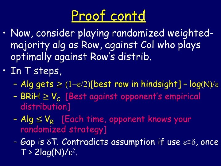
Proof contd •