THE VIRTUAL FIELDS METHOD Introduction and Overview Professor

THE VIRTUAL FIELDS METHOD Introduction and Overview Professor Fabrice PIERRON LMPF Research Group, ENSAM Châlons en Champagne, France Paris Châlons en Champagne

A bit of history

A bit of history 1989 – First paper in “Comptes rendus de l’académie des sciences” (principle) 1990 – Ph. D thesis of Michel GRÉDIAC (thin anisotropic plates, including experiments) 1994 – First collaboration between FP & MG (anisotropic in-plane properties, shear) 1996 – 98: First application in dynamics (vibration of thin plates, exp. & num. ) 1998 – 2000: Series of work on in-plane elastic stiffnesses of composites (exp. & num. ) 2001: first attempt at a non-linear law (anisotropic) 2002 – 04: Significant progress on virtual fields selection in elasticity (special virtual fields, minimization of noise effects) 3

A bit of history 2003: First application in vibration with damping (thin plates) 2005 – 06: Convincing experimental results (in-plane anisotropic composite stiffnesses) 2006 – First application to elasto-plasticity 2006: Theoretical framework in elasticity (relation between FEMU and VFM) 2006: Optimisation of test configuration (with Airbus UK) 2006: First application on heterogeneous materials – stiffness contrast in impacted composite plates (with Bristol Univ. ) 4

A bit of history 2007: Application to elastography (MRI) 2007: First application to viscoplasticity (coll. M. A. Sutton) 2007: First application to heterogeneous plasticity (FSW joints) Ongoing Application to 3 D bulk measurements (composites, biomechanics), project with Loughborough university (Prof. J. M. Huntley, Dr P. D. Ruiz) Optimisation of virtual fields in plasticity Friction Stir Welds (collaboration with ONERA, France) Development of a user-oriented software: CAMFIT 5

The principle of virtual work

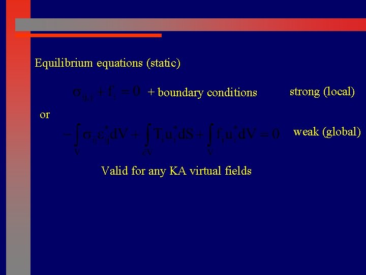
Equilibrium equations (static) + boundary conditions strong (local) or weak (global) Valid for any KA virtual fields

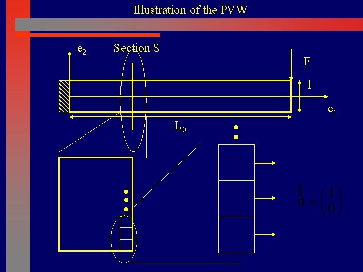
Illustration of the PVW e 2 Section S F l e 1 L 0

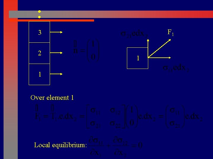
F 1 3 2 1 Over element 1 Local equilibrium: 1

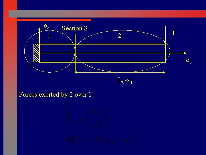
e 2 1 Section S 2 F e 1 L 0 -x 1 Forces exerted by 2 over 1

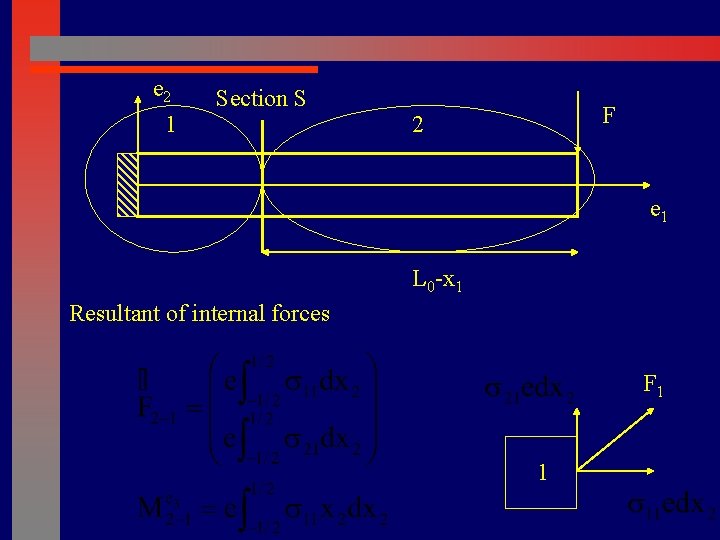
e 2 1 Section S F 2 e 1 L 0 -x 1 Resultant of internal forces F 1 1

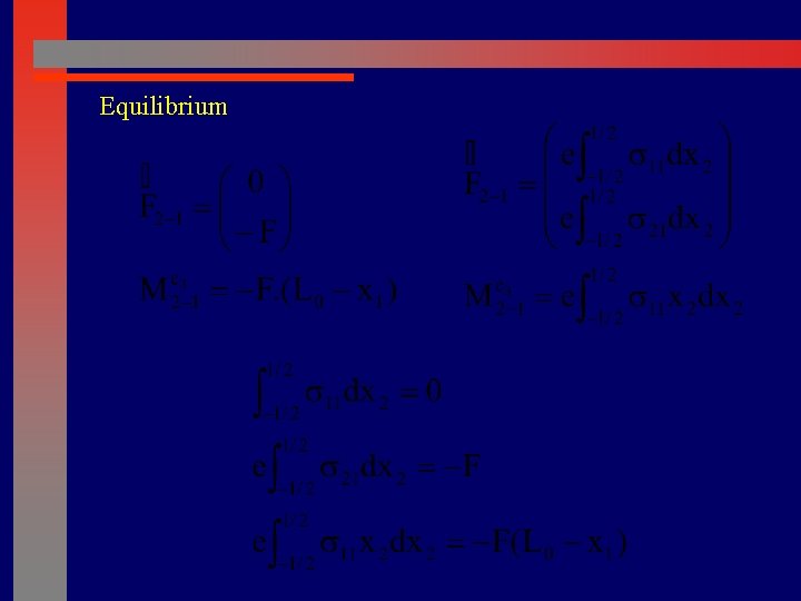
Equilibrium

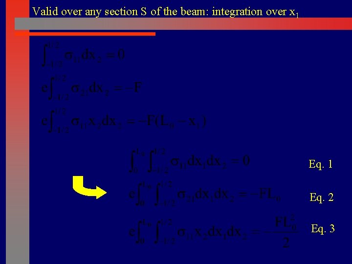
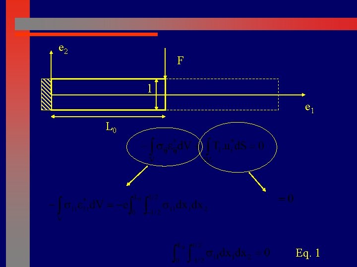
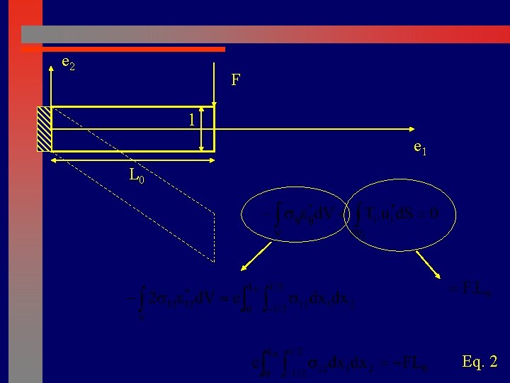
Valid over any section S of the beam: integration over x 1 Eq. 2 Eq. 3

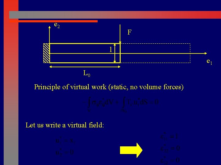
e 2 F l e 1 L 0 Principle of virtual work (static, no volume forces) Let us write a virtual field:

e 2 F l e 1 L 0 Eq. 1

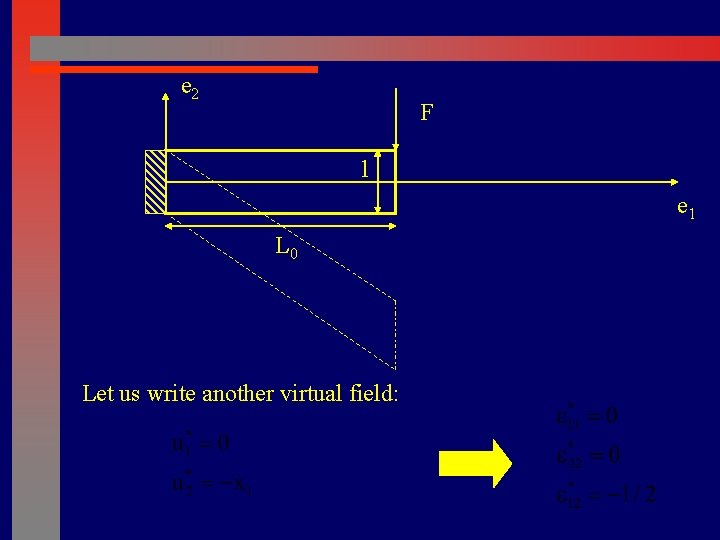
e 2 F l e 1 L 0 Let us write another virtual field:

e 2 F l e 1 L 0 Eq. 2

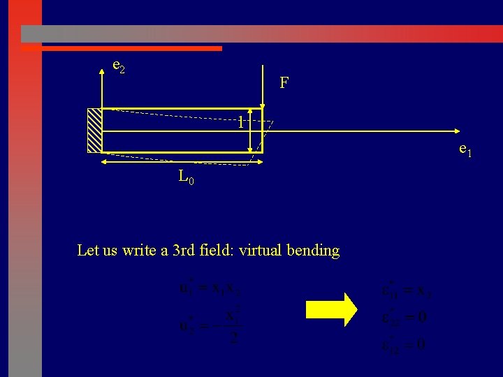
e 2 F l e 1 L 0 Let us write a 3 rd field: virtual bending

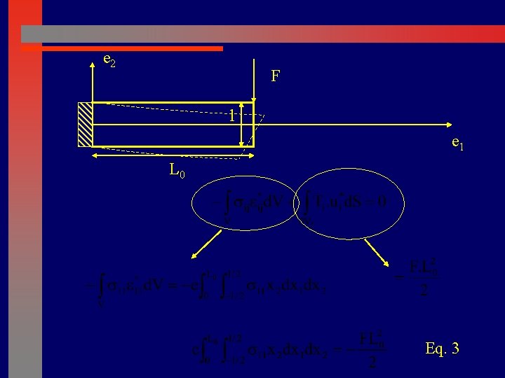
e 2 F l e 1 L 0 Eq. 3

The Virtual Fields Method

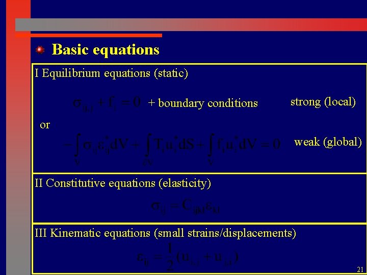
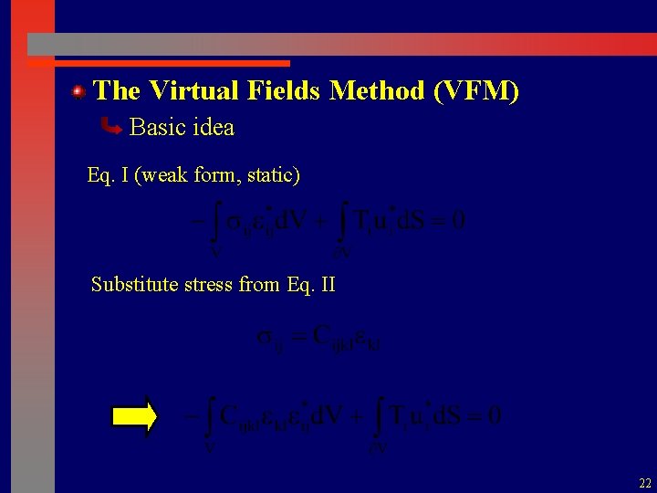
Basic equations I Equilibrium equations (static) + boundary conditions strong (local) or weak (global) II Constitutive equations (elasticity) III Kinematic equations (small strains/displacements) 21

The Virtual Fields Method (VFM) Basic idea Eq. I (weak form, static) Substitute stress from Eq. II 22

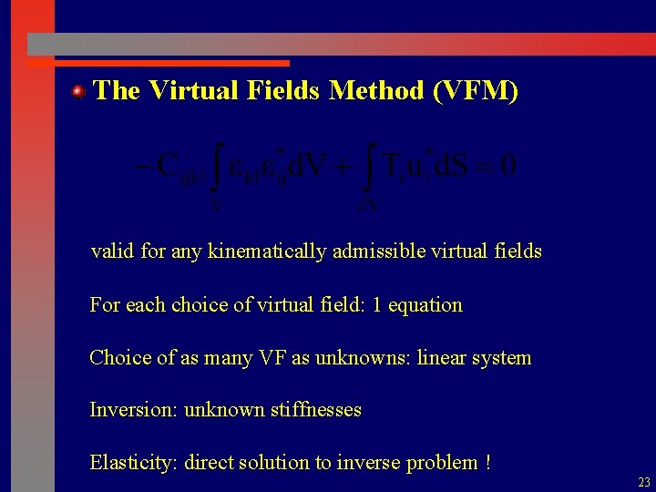
The Virtual Fields Method (VFM) valid for any kinematically admissible virtual fields For each choice of virtual field: 1 equation Choice of as many VF as unknowns: linear system Inversion: unknown stiffnesses Elasticity: direct solution to inverse problem ! 23

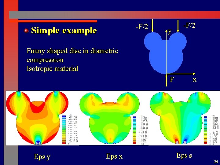
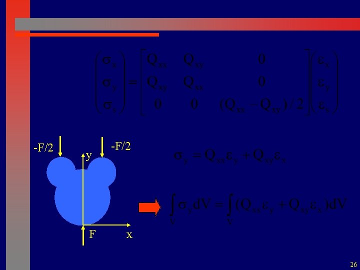
-F/2 Simple example y -F/2 Fuuny shaped disc in diametric compression Isotropic material x F Eps y Eps x Eps s 24

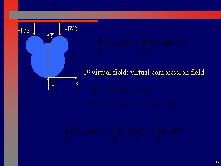
-F/2 y -F/2 1 st virtual field: virtual compression field F x 25

-F/2 y F -F/2 x 26

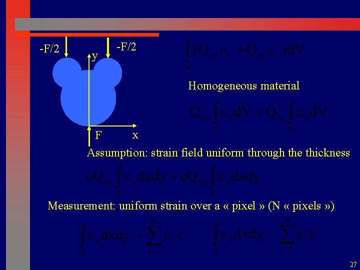
-F/2 y -F/2 Homogeneous material x F Assumption: strain field uniform through the thickness Measurement: uniform strain over a « pixel » (N « pixels » ) 27

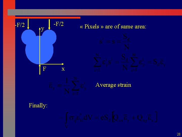
-F/2 y F -F/2 « Pixels » are of same area: x Average strain Finally: 28

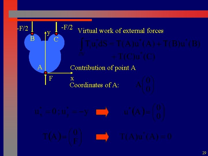
-F/2 y B A -F/2 Virtual work of external forces C Contribution of point A F x Coordinates of A: 29

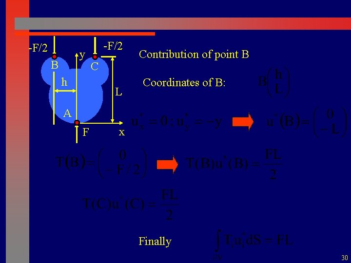
-F/2 y B h -F/2 C L Contribution of point B Coordinates of B: A F x Finally 30

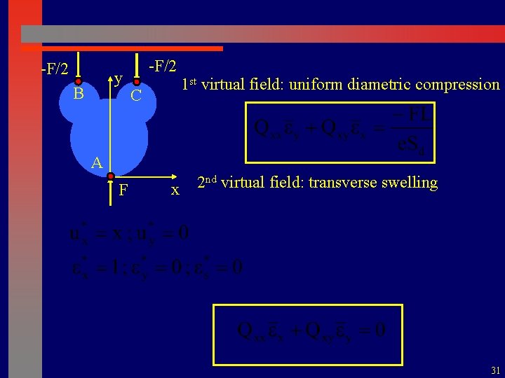
-F/2 y B -F/2 C 1 st virtual field: uniform diametric compression A F x 2 nd virtual field: transverse swelling 31

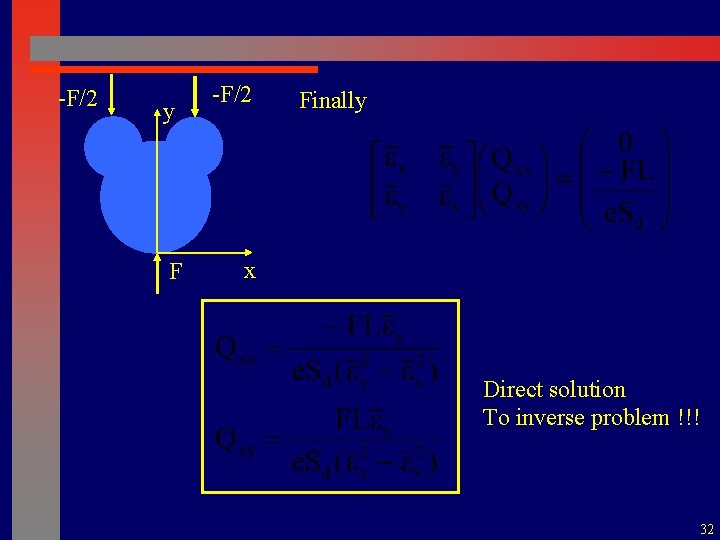
-F/2 y F -F/2 Finally x Direct solution To inverse problem !!! 32

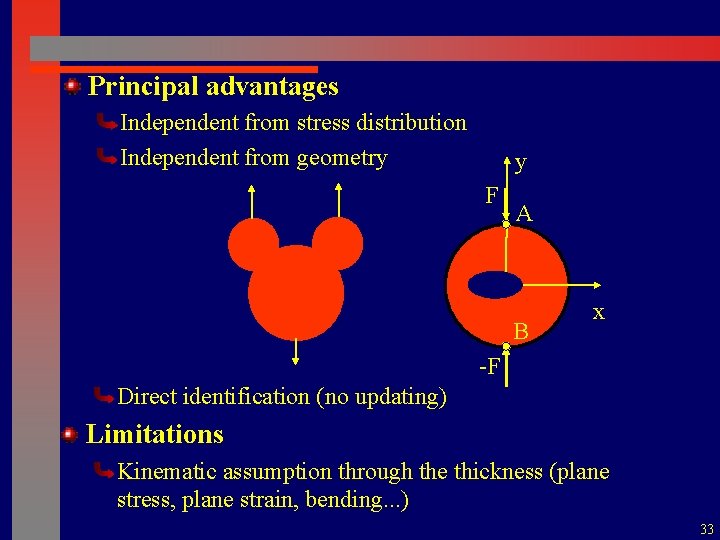
Principal advantages Independent from stress distribution Independent from geometry y F A B x -F Direct identification (no updating) Limitations Kinematic assumption through the thickness (plane stress, plane strain, bending. . . ) 33

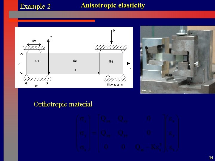
Example 2 Anisotropic elasticity Orthotropic material 34

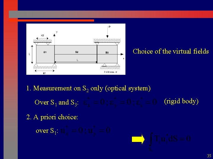
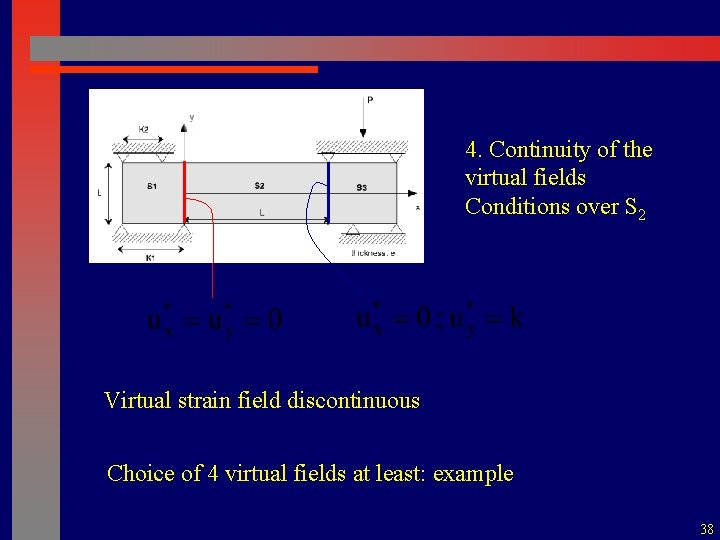
Choice of the virtual fields 1. Measurement on S 2 only (optical system) Over S 1 and S 3: (rigid body) 2. A priori choice: over S 1: 35

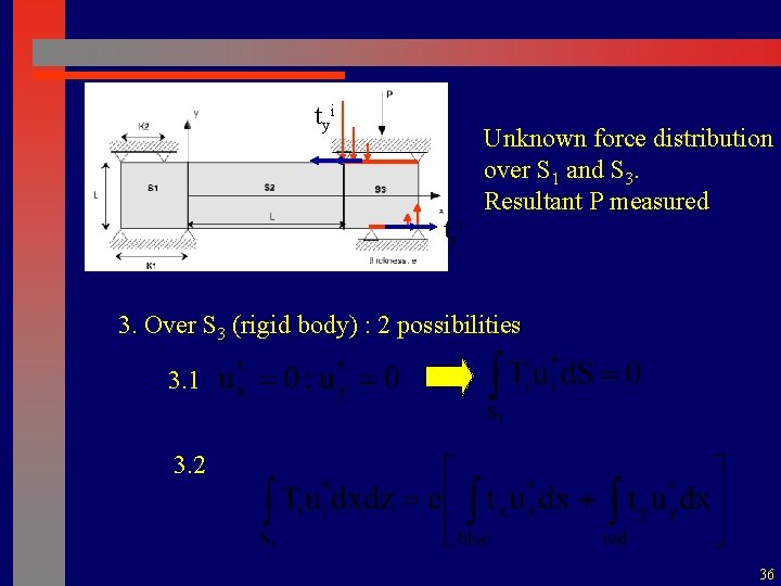
tyi txi Unknown force distribution over S 1 and S 3. Resultant P measured 3. Over S 3 (rigid body) : 2 possibilities 3. 1 3. 2 36

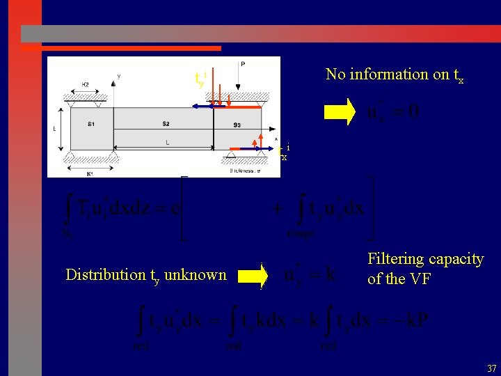
No information on tx tyi txi Distribution ty unknown Filtering capacity of the VF 37

4. Continuity of the virtual fields Conditions over S 2 Virtual strain field discontinuous Choice of 4 virtual fields at least: example 38

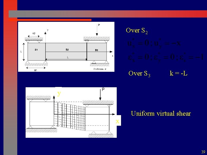
Over S 2 Over S 3 k = -L y x Uniform virtual shear 39

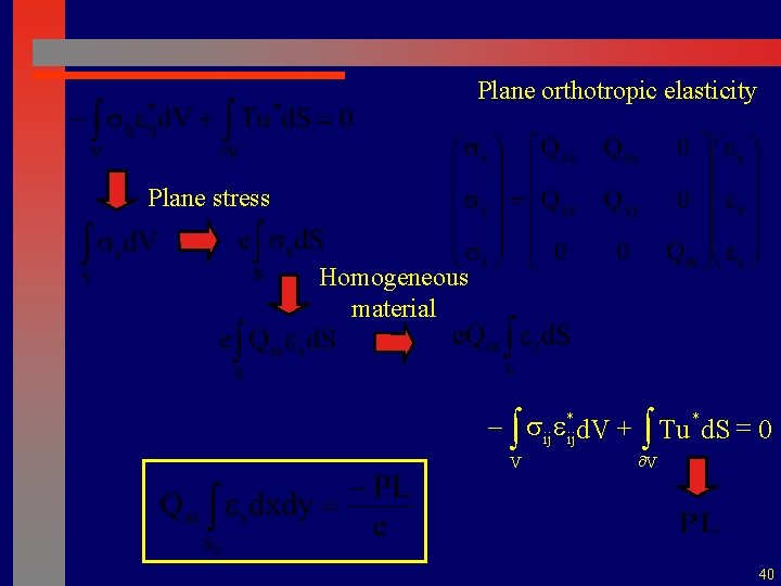
Plane orthotropic elasticity Plane stress Homogeneous material - ò s ije*ijd. V + ò Tu *d. S = 0 V ¶V 40

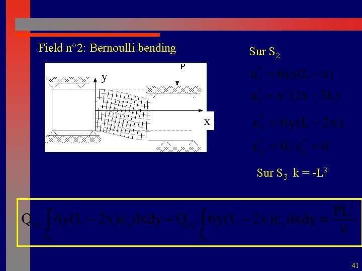
Field n° 2: Bernoulli bending Sur S 2 y x Sur S 3 k = -L 3 41

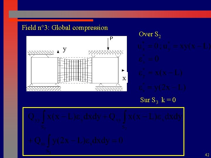
Field n° 3: Global compression Over S 2 y x Sur S 3 k = 0 42

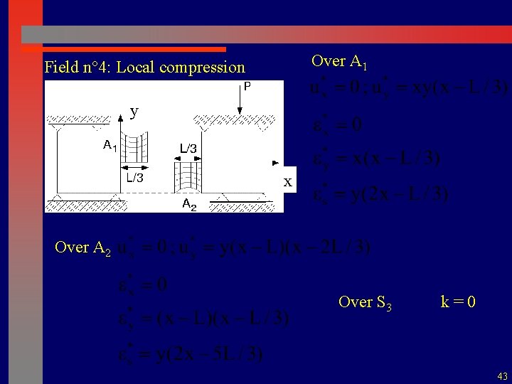
Over A 1 Field n° 4: Local compression y x Over A 2 Over S 3 k = 0 43

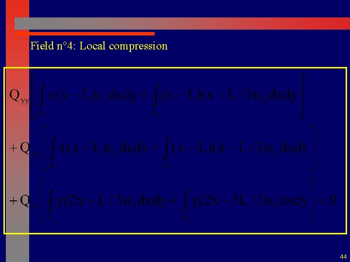
Field n° 4: Local compression 44

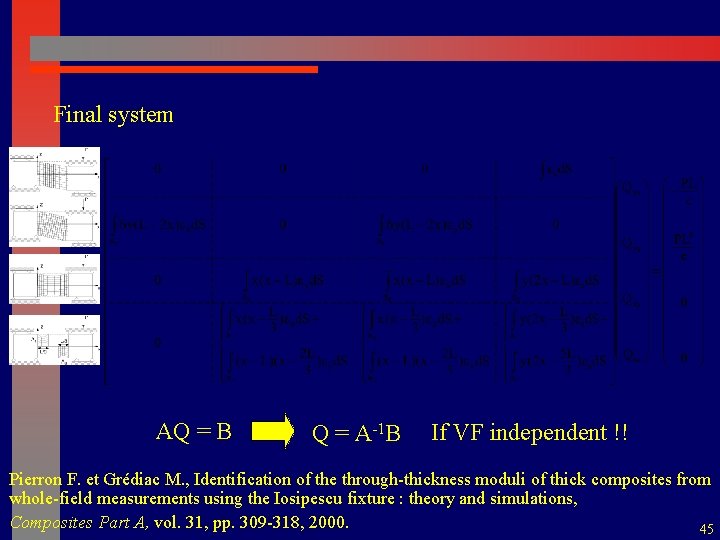
Final system AQ = B Q = A-1 B If VF independent !! Pierron F. et Grédiac M. , Identification of the through-thickness moduli of thick composites from whole-field measurements using the Iosipescu fixture : theory and simulations, Composites Part A, vol. 31, pp. 309 -318, 2000. 45

Experimental examples in linear elasticity 46

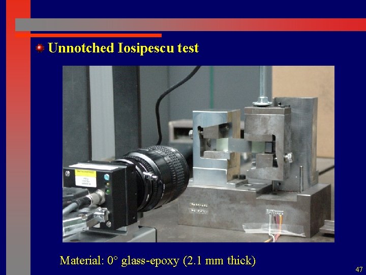
Unnotched Iosipescu test Material: 0° glass-epoxy (2. 1 mm thick) 47

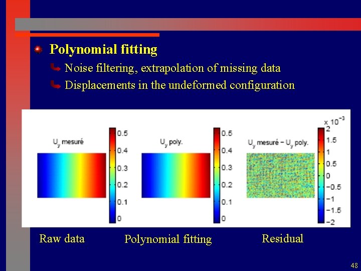
Polynomial fitting Noise filtering, extrapolation of missing data Displacements in the undeformed configuration Raw data Polynomial fitting Residual 48

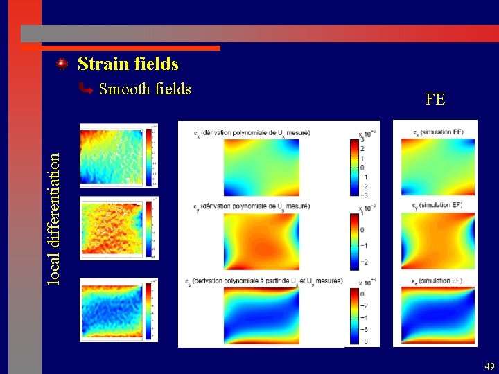
Strain fields FE local differentiation Smooth fields 49

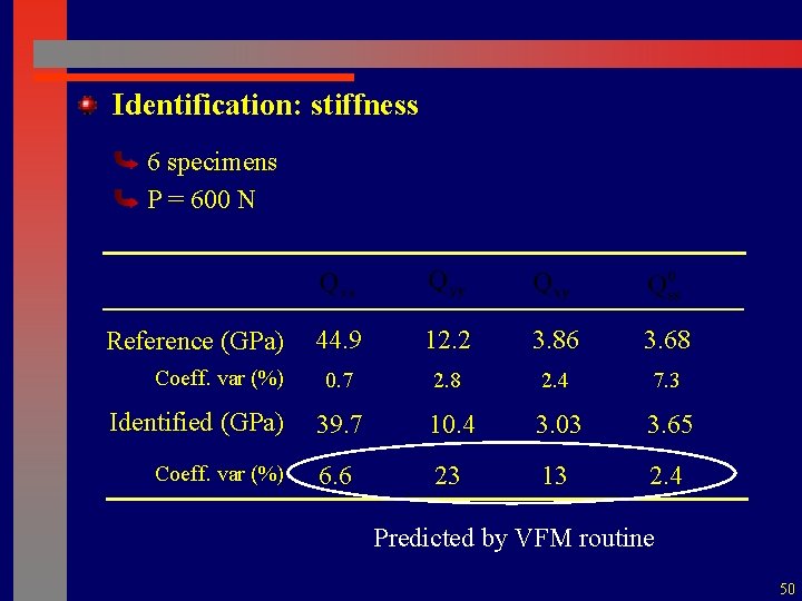
Identification: stiffness 6 specimens P = 600 N Reference (GPa) Coeff. var (%) Identified (GPa) Coeff. var (%) 44. 9 12. 2 3. 86 3. 68 0. 7 2. 8 2. 4 7. 3 39. 7 10. 4 3. 03 3. 65 6. 6 23 13 2. 4 Predicted by VFM routine 50

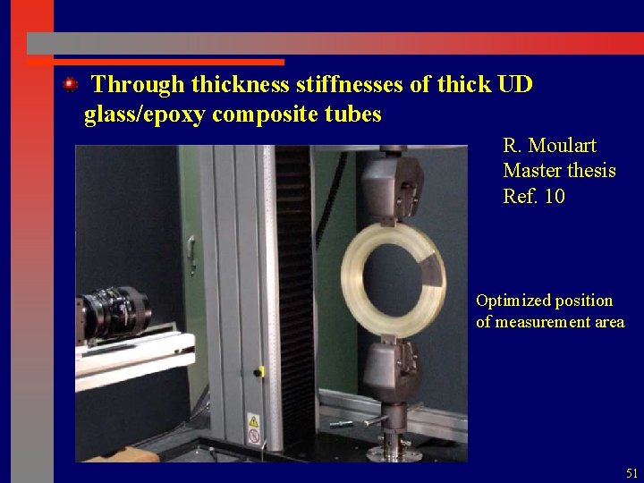
Through thickness stiffnesses of thick UD glass/epoxy composite tubes R. Moulart Master thesis Ref. 10 Optimized position of measurement area 51

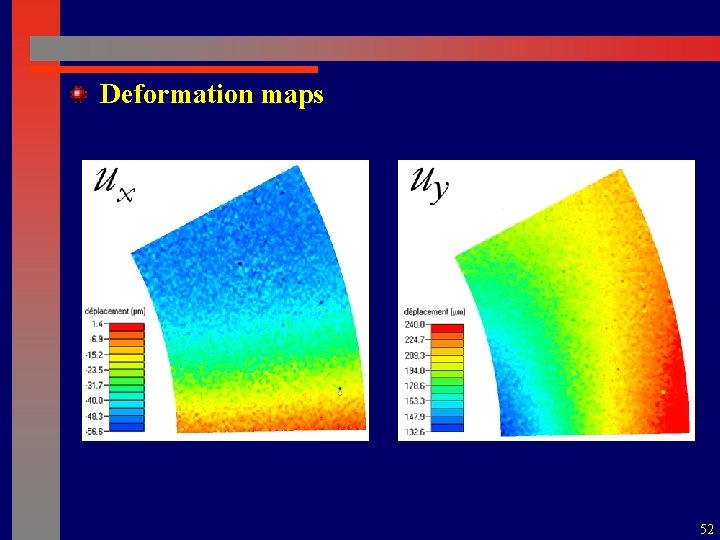
Deformation maps 52

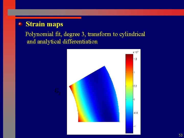
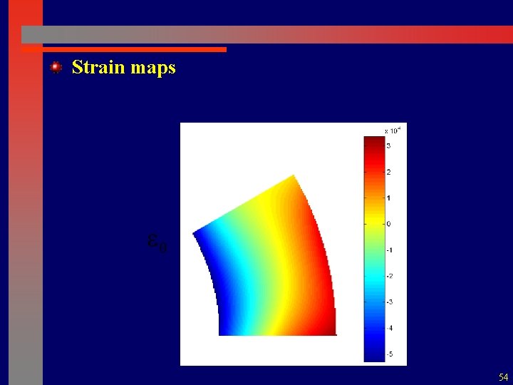
Strain maps Polynomial fit, degree 3, transform to cylindrical and analytical differentiation 53

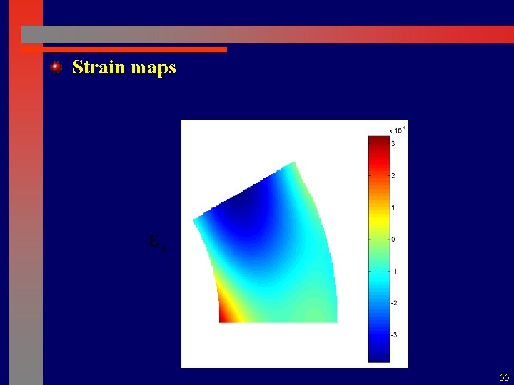
Strain maps 54

Strain maps 55

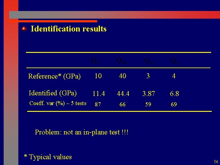
Identification results Reference* (GPa) 10 40 3 4 Identified (GPa) 11. 4 44. 4 3. 87 6. 8 87 66 59 69 Coeff. var (%) – 5 tests Problem: not an in-plane test !!! * Typical values 56

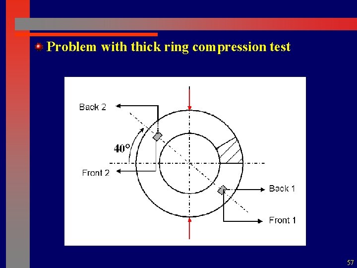
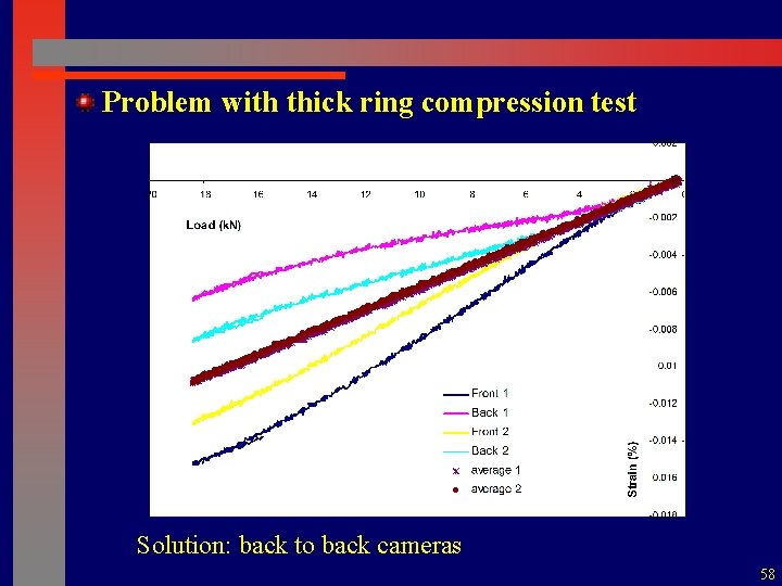
Problem with thick ring compression test 57

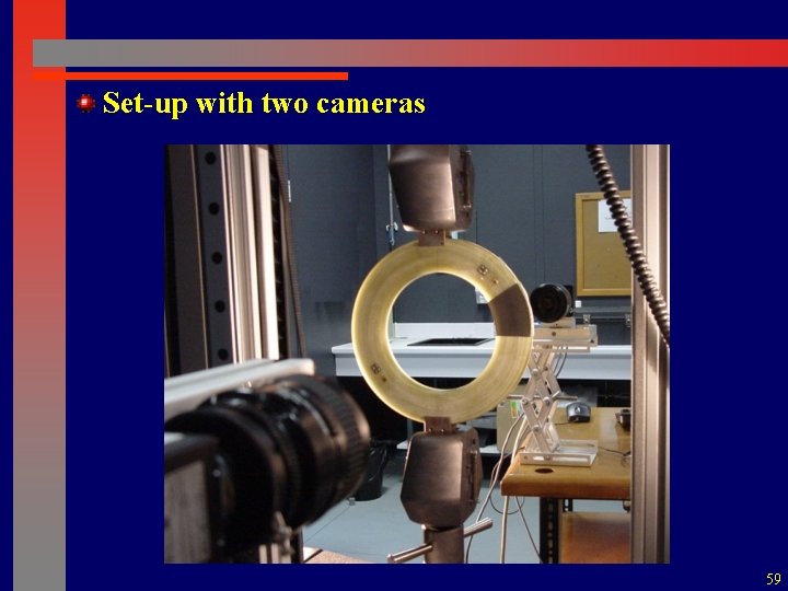
Problem with thick ring compression test Solution: back to back cameras 58

Set-up with two cameras 59

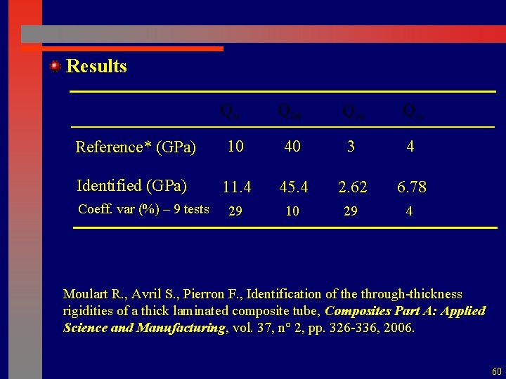
Results Reference* (GPa) 10 40 3 4 Identified (GPa) 11. 4 45. 4 2. 62 6. 78 29 10 29 4 Coeff. var (%) – 9 tests Moulart R. , Avril S. , Pierron F. , Identification of the through-thickness rigidities of a thick laminated composite tube, Composites Part A: Applied Science and Manufacturing, vol. 37, n° 2, pp. 326 -336, 2006. 60

ACKNOWLEDGEMENTS Professor Michel GREDIAC Blaise Pascal University, France Colleagues and students from my research group: Dr Stéphane Avril, Dr Alain Giraudeau, Dr René Rotinat Dr Hocine Chalal, Mr Baoqiao Guo, Dr Yannick Pannier, Mr Raphaël Moulart French CNRS network (GDR): « full-field measurements and identification in solid mechanics » 61

ACKNOWLEDGEMENTS Funding French Ministry for Research French National Research Agency (ANR) Champagne Ardenne Regional Council Engineering and Physical Sciences Research Council (UK) Airbus UK 62