The use of models in biology Bas Kooijman

The use of models in biology Bas Kooijman Afdeling Theoretische Biologie Vrije Universiteit Amsterdam http: //www. bio. vu. nl/thb/ Bas@bio. vu. nl Eindhoven, 2003/02/15

Modelling 1 • model: scientific statement in mathematical language “all models are wrong, some are useful” • aims: structuring thought; the single most useful property of models: “a model is not more than you put into it” how do factors interact? (machanisms/consequences) design of experiments, interpretation of results inter-, extra-polation (prediction) decision/management (risk analysis)

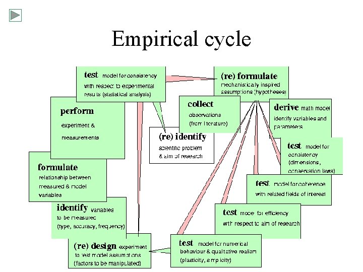
Empirical cycle

Modelling 2 • language errors: mathematical, dimensions, conservation laws • properties: generic (with respect to application) realistic (precision) simple (math. analysis, aid in thinking) plasticity in parameters (support, testability) • ideals: assumptions for mechanisms (coherence, consistency) distinction action variables/meausered quantities core/auxiliary theory

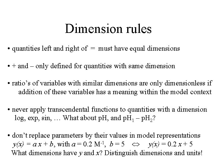
Dimension rules • quantities left and right of = must have equal dimensions • + and – only defined for quantities with same dimension • ratio’s of variables with similar dimensions are only dimensionless if addition of these variables has a meaning within the model context • never apply transcendental functions to quantities with a dimension log, exp, sin, … What about p. H, and p. H 1 – p. H 2? • don’t replace parameters by their values in model representations y(x) = a x + b, with a = 0. 2 M-1, b = 5 y(x) = 0. 2 x + 5 What dimensions have y and x? Distinguish dimensions and units!

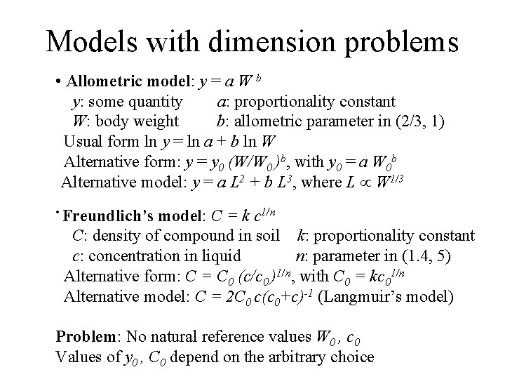
Models with dimension problems • Allometric model: y = a W b y: some quantity a: proportionality constant W: body weight b: allometric parameter in (2/3, 1) Usual form ln y = ln a + b ln W Alternative form: y = y 0 (W/W 0 )b, with y 0 = a W 0 b Alternative model: y = a L 2 + b L 3, where L W 1/3 • Freundlich’s model: C = k c 1/n C: density of compound in soil k: proportionality constant c: concentration in liquid n: parameter in (1. 4, 5) Alternative form: C = C 0 (c/c 0 )1/n, with C 0 = kc 01/n Alternative model: C = 2 C 0 c(c 0+c)-1 (Langmuir’s model) Problem: No natural reference values W 0 , c 0 Values of y 0 , C 0 depend on the arbitrary choice

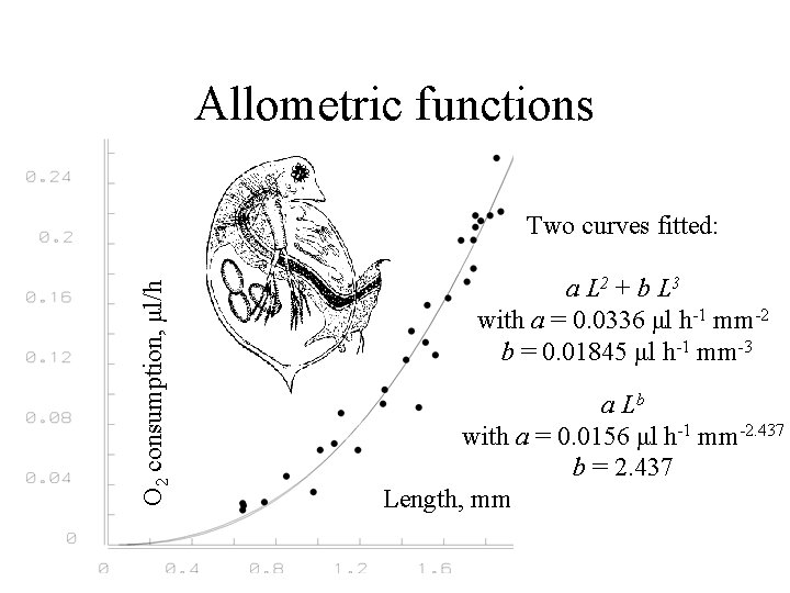
Allometric functions O 2 consumption, μl/h Two curves fitted: a L 2 + b L 3 with a = 0. 0336 μl h-1 mm-2 b = 0. 01845 μl h-1 mm-3 a Lb with a = 0. 0156 μl h-1 mm-2. 437 b = 2. 437 Length, mm

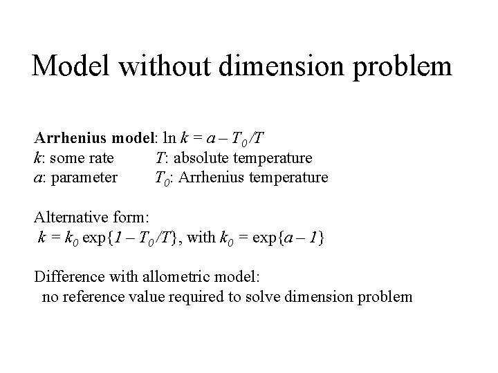
Model without dimension problem Arrhenius model: ln k = a – T 0 /T k: some rate T: absolute temperature a: parameter T 0: Arrhenius temperature Alternative form: k = k 0 exp{1 – T 0 /T}, with k 0 = exp{a – 1} Difference with allometric model: no reference value required to solve dimension problem

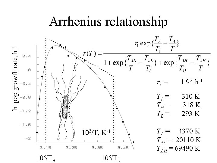
ln pop growth rate, h-1 Arrhenius relationship 103/T, K-1 103/TH 103/TL r 1 = 1. 94 h-1 T 1 = TH = TL = 310 K 318 K 293 K TA = 4370 K TAL = 20110 K TAH = 69490 K

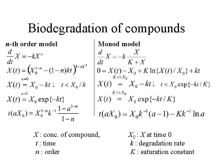
Biodegradation of compounds n-th order model Monod model ; X : conc. of compound, t : time n : order ; X 0 : X at time 0 k : degradation rate K : saturation constant

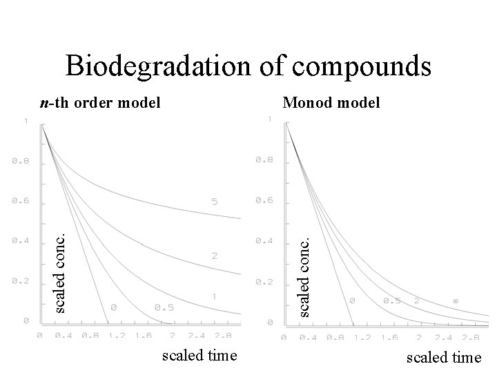
Biodegradation of compounds Monod model scaled conc. n-th order model scaled time

Plasticity in parameters If plasticity of shapes of y(x|a) is large as function of a: • little problems in estimating value of a from {xi, yi}i (small confidence intervals) • little support from data for underlying assumptions (if data were different: other parameter value results, but still a good fit, so no rejection of assumption)

Stochastic vs deterministic models Only stochastic models can be tested against experimental data Standard way to extend deterministic model to stochastic one: regression model: y(x| a, b, . . ) = f(x|a, b, . . ) + e, with e N(0, 2) Originates from physics, where e stands for measurement error Problem: deviations from model are frequently not measurement errors Alternatives: • deterministic systems with stochastic inputs • differences in parameter values between individuals Problem: parameter estimation methods become very complex

Statistics Deals with • estimation of parameter values, and confidence in these values • tests of hypothesis about parameter values differs a parameter value from a known value? differ parameter values between two samples? Deals NOT with • does model 1 fit better than model 2 if model 1 is not a special case of model 2 Statistical methods assume that the model is given (Non-parametric methods only use some properties of the given model, rather than its full specification)

Dynamic systems Defined by simultaneous behaviour of input, state variable, output Supply systems: input + state variables output Demand systems input state variables + output Real systems: mixtures between supply & demand systems Constraints: mass, energy balance equations State variables: span a state space behaviour: usually set of ode’s with parameters Trajectory: map of behaviour state vars in state space Parameters: constant, functions of time, functions of modifying variables compound parameters: functions of parameters

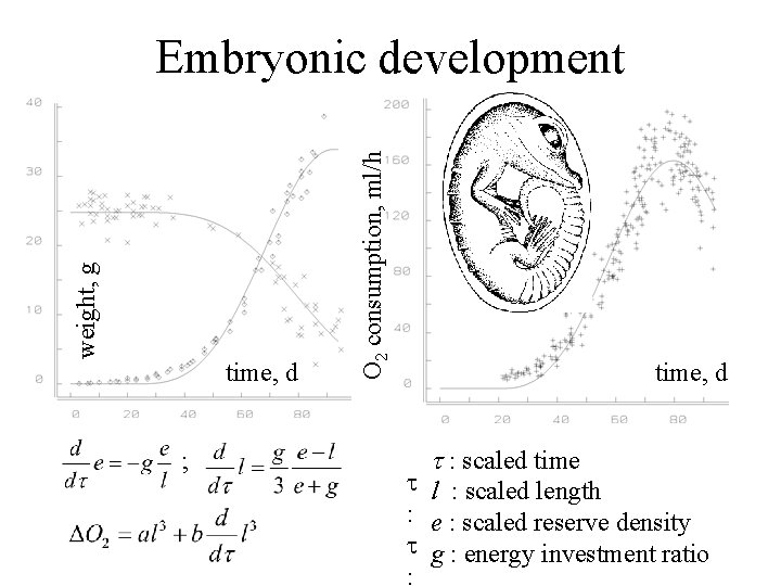
time, d ; O 2 consumption, ml/h weight, g Embryonic development time, d : scaled time l : scaled length : e : scaled reserve density g : energy investment ratio :

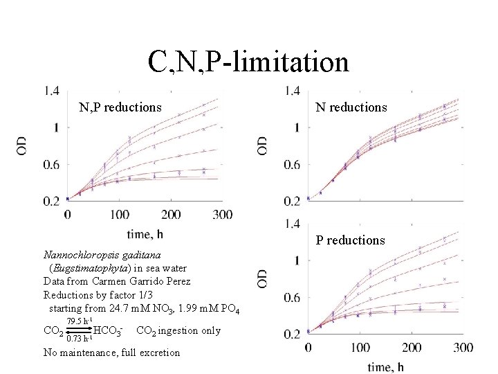
C, N, P-limitation N, P reductions N reductions P reductions Nannochloropsis gaditana (Eugstimatophyta) in sea water Data from Carmen Garrido Perez Reductions by factor 1/3 starting from 24. 7 m. M NO 3, 1. 99 m. M PO 4 CO 2 79. 5 h-1 0. 73 h-1 HCO 3 - CO 2 ingestion only No maintenance, full excretion

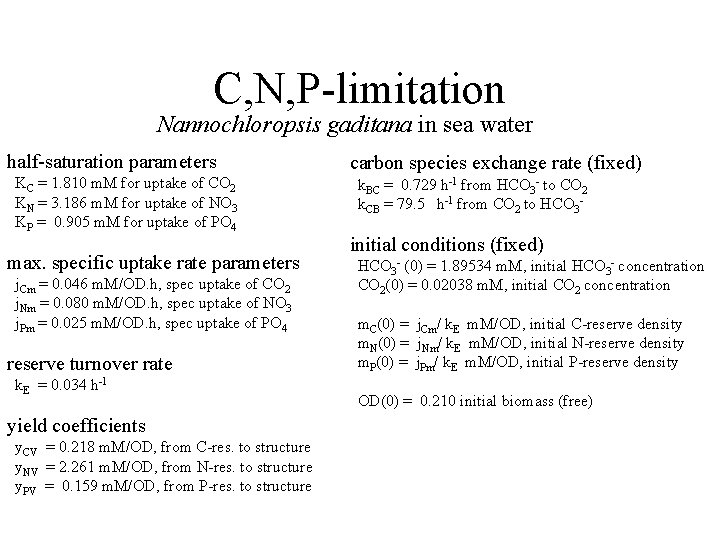
C, N, P-limitation Nannochloropsis gaditana in sea water half-saturation parameters KC = 1. 810 m. M for uptake of CO 2 KN = 3. 186 m. M for uptake of NO 3 KP = 0. 905 m. M for uptake of PO 4 max. specific uptake rate parameters j. Cm = 0. 046 m. M/OD. h, spec uptake of CO 2 j. Nm = 0. 080 m. M/OD. h, spec uptake of NO 3 j. Pm = 0. 025 m. M/OD. h, spec uptake of PO 4 reserve turnover rate k. E = 0. 034 h-1 yield coefficients y. CV = 0. 218 m. M/OD, from C-res. to structure y. NV = 2. 261 m. M/OD, from N-res. to structure y. PV = 0. 159 m. M/OD, from P-res. to structure carbon species exchange rate (fixed) k. BC = 0. 729 h-1 from HCO 3 - to CO 2 k. CB = 79. 5 h-1 from CO 2 to HCO 3 - initial conditions (fixed) HCO 3 - (0) = 1. 89534 m. M, initial HCO 3 - concentration CO 2(0) = 0. 02038 m. M, initial CO 2 concentration m. C(0) = j. Cm/ k. E m. M/OD, initial C-reserve density m. N(0) = j. Nm/ k. E m. M/OD, initial N-reserve density m. P(0) = j. Pm/ k. E m. M/OD, initial P-reserve density OD(0) = 0. 210 initial biomass (free)

Further reading Basic methods of theoretical biology freely downloadable document on methods http: //www. bio. vu. nl/thb/course/tb/ Data-base with examples, exercises under construction Dynamic Energy Budget theory http: //www. bio. vu. nl/thb/deb/