The University of Iowa 22 c 296 Automated

The University of Iowa 22 c: 296 Automated Software Verification Modeling Software Systems for Analysis Copyright 2003 -04, Doron Peled and Cesare Tinelli. These notes are based on a set of lecture notes originally developed by Doron Peled at the University of Warwick. These notes are copyrighted materials and may not be used in other course settings outside of the University of Iowa in their current form or modified form without the express written permission of the copyright holders. During this course, students are prohibited from selling notes to or being paid for taking notes by any person or commercial firm without the express written permission of the copyright holders.

Modelling n n n Modelling: representing a system in terms mathematical objects that reflect the system’s relevant properties. Modelling often involves abstraction, to focus on main properties and manage complexity (Modelling is also required because mathematical methods cannot handle physical systems, only abstractions of them. )

Modelling n Modelling can be applied to existing systems, to reason about them after they have been built (good) n future systems, to drive the design and construction of a system, and catch errors at the model level already (better) n

Modelling n n Modelling is a subtle task. Main issues: n n n Selection of relevant properties Right level of abstraction If not done properly, verification of the model may not carry over to the actual system (missed errors, spurious errors)

Modelling and specification for verification How to specify what the software is supposed to do? n How to model it in a way that allows us to check it? n

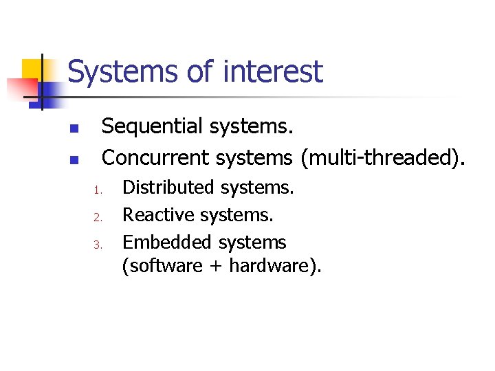
Systems of interest n n Sequential systems. Concurrent systems (multi-threaded). 1. 2. 3. Distributed systems. Reactive systems. Embedded systems (software + hardware).

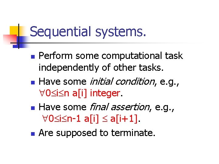
Sequential systems. n n Perform some computational task independently of other tasks. Have some initial condition, e. g. , 0 i n a[i] integer. Have some final assertion, e. g. , 0 i n-1 a[i] a[i+1]. Are supposed to terminate.

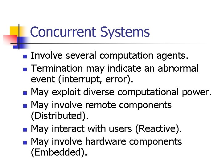
Concurrent Systems n n n Involve several computation agents. Termination may indicate an abnormal event (interrupt, error). May exploit diverse computational power. May involve remote components (Distributed). May interact with users (Reactive). May involve hardware components (Embedded).

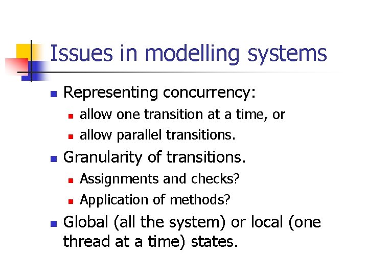
Issues in modelling systems n Representing concurrency: n n n Granularity of transitions. n n n allow one transition at a time, or allow parallel transitions. Assignments and checks? Application of methods? Global (all the system) or local (one thread at a time) states.

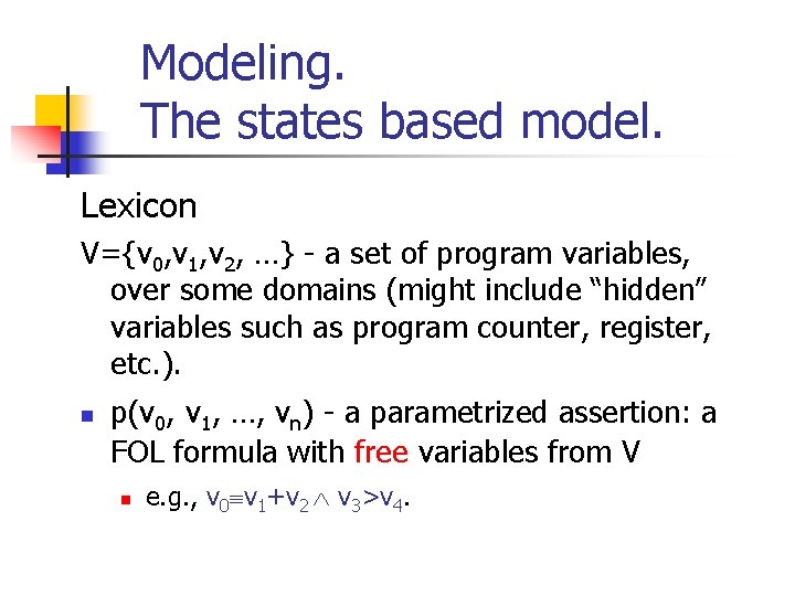
Modeling. The states based model. Lexicon V={v 0, v 1, v 2, …} - a set of program variables, over some domains (might include “hidden” variables such as program counter, register, etc. ). n p(v 0, v 1, …, vn) - a parametrized assertion: a FOL formula with free variables from V n e. g. , v 0 v 1+v 2 v 3>v 4.

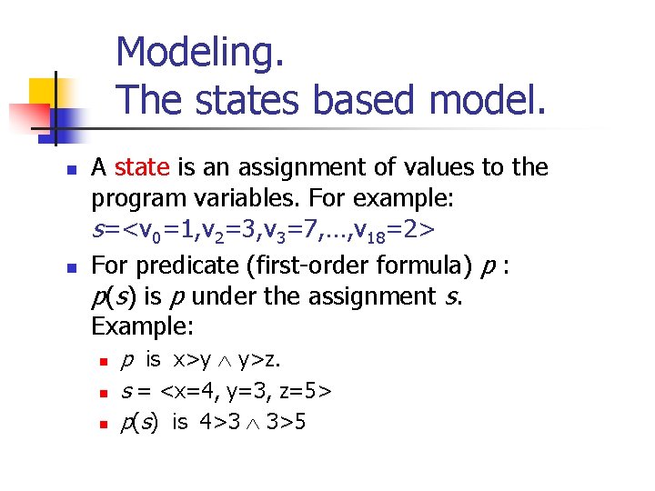
Modeling. The states based model. n n A state is an assignment of values to the program variables. For example: s=<v 0=1, v 2=3, v 3=7, …, v 18=2> For predicate (first-order formula) p : p(s) is p under the assignment s. Example: n n n p is x>y y>z. s = <x=4, y=3, z=5> p(s) is 4>3 3>5

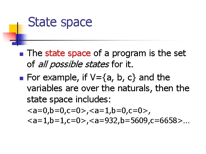
State space n n The state space of a program is the set of all possible states for it. For example, if V={a, b, c} and the variables are over the naturals, then the state space includes: <a=0, b=0, c=0>, <a=1, b=1, c=0>, <a=932, b=5609, c=6658>…

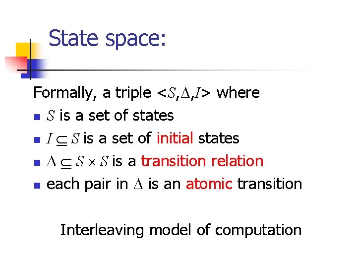
State space: Formally, a triple <S, , I> where n S is a set of states n I S is a set of initial states n S S is a transition relation n each pair in is an atomic transition Interleaving model of computation

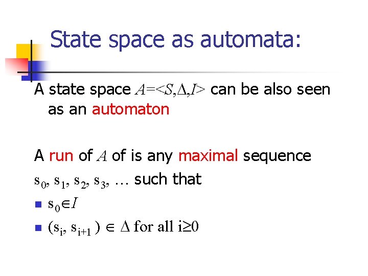
State space as automata: A state space A=<S, , I> can be also seen as an automaton A run of A of is any maximal sequence s 0, s 1, s 2, s 3, … such that n s 0 I n (si, si+1 ) for all i 0

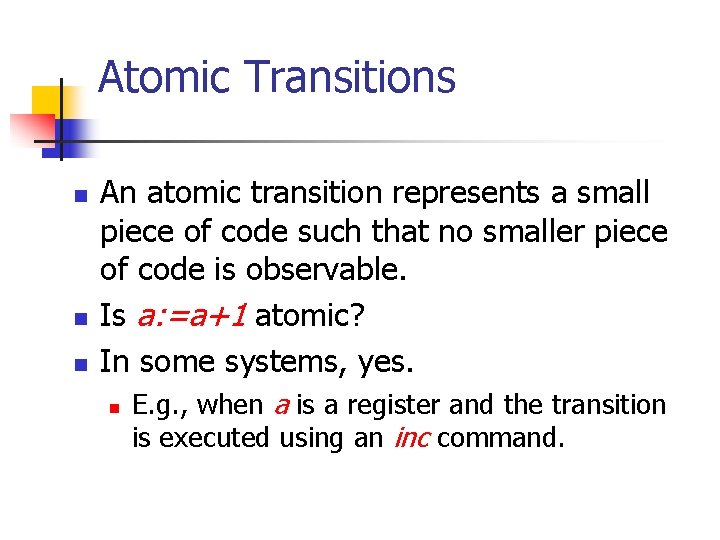
Atomic Transitions n n n An atomic transition represents a small piece of code such that no smaller piece of code is observable. Is a: =a+1 atomic? In some systems, yes. n E. g. , when a is a register and the transition is executed using an inc command.

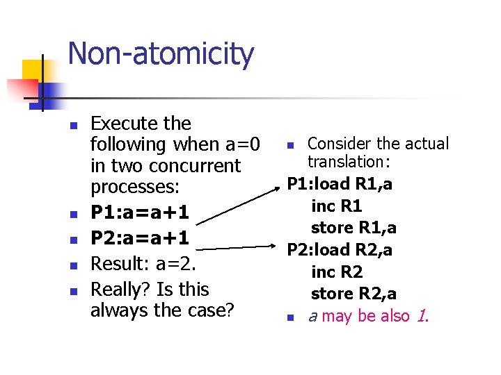
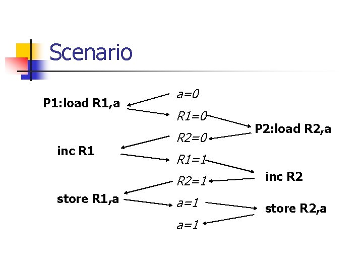
Non-atomicity n n n Execute the following when a=0 in two concurrent processes: P 1: a=a+1 P 2: a=a+1 Result: a=2. Really? Is this always the case? Consider the actual translation: P 1: load R 1, a inc R 1 store R 1, a P 2: load R 2, a inc R 2 store R 2, a n a may be also 1. n

Scenario P 1: load R 1, a inc R 1 store R 1, a a=0 R 1=0 R 2=0 P 2: load R 2, a R 1=1 R 2=1 inc R 2 a=1 store R 2, a a=1

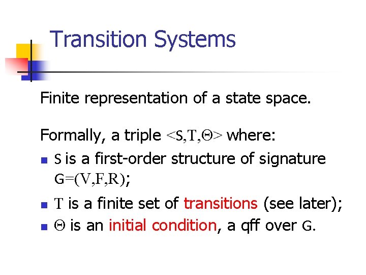
Transition Systems Finite representation of a state space. Formally, a triple <S, T, > where: n S is a first-order structure of signature G=(V, F, R); n n T is a finite set of transitions (see later); is an initial condition, a qff over G.

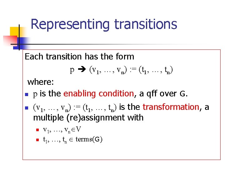
Representing transitions Each transition has the form p (v 1, …, vn) : = (t 1, …, tn) where: n p is the enabling condition, a qff over G. n (v 1, …, vn) : = (t 1, …, tn) is the transformation, a multiple (re)assignment with n n v 1, …, vn V t 1, …, tn terms(G)

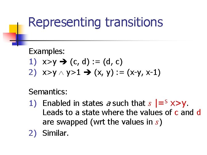
Representing transitions Examples: 1) x>y (c, d) : = (d, c) 2) x>y y>1 (x, y) : = (x-y, x-1) Semantics: 1) Enabled in states a such that s |=S x>y. Leads to a state where the values of c and d are swapped (wrt the values in s) 2) Similar.

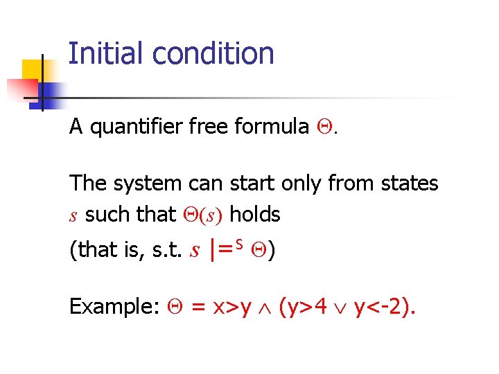
Initial condition A quantifier free formula . The system can start only from states s such that (s) holds (that is, s. t. s |=S ) Example: = x>y (y>4 y<-2).

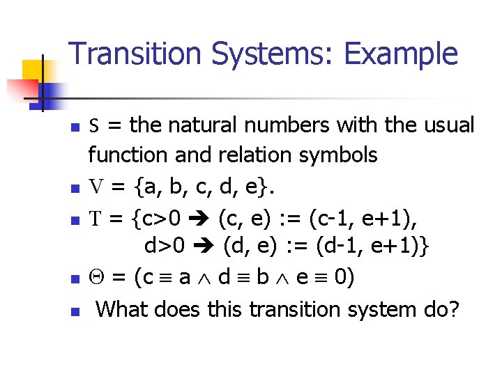
Transition Systems: Example n n n S = the natural numbers with the usual function and relation symbols V = {a, b, c, d, e}. T = {c>0 (c, e) : = (c-1, e+1), d>0 (d, e) : = (d-1, e+1)} = (c a d b e 0) What does this transition system do?

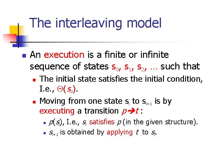
The interleaving model n An execution is a finite or infinite sequence of states s 0, s 1, s 2, … such that n n The initial state satisfies the initial condition, I. e. , (s 0). Moving from one state si to si+1 is by executing a transition p t : n n p(si), I. e. , si satisfies p (in the given structure). si+1 is obtained by applying t to si.

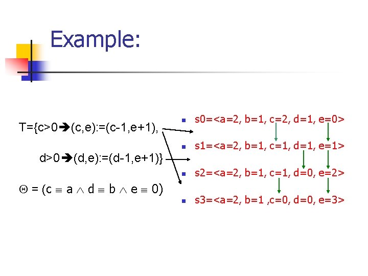
Example: T={c>0 (c, e): =(c-1, e+1), n s 0=<a=2, b=1, c=2, d=1, e=0> n s 1=<a=2, b=1, c=1, d=1, e=1> n s 2=<a=2, b=1, c=1, d=0, e=2> n s 3=<a=2, b=1 , c=0, d=0, e=3> d>0 (d, e): =(d-1, e+1)} = (c a d b e 0)

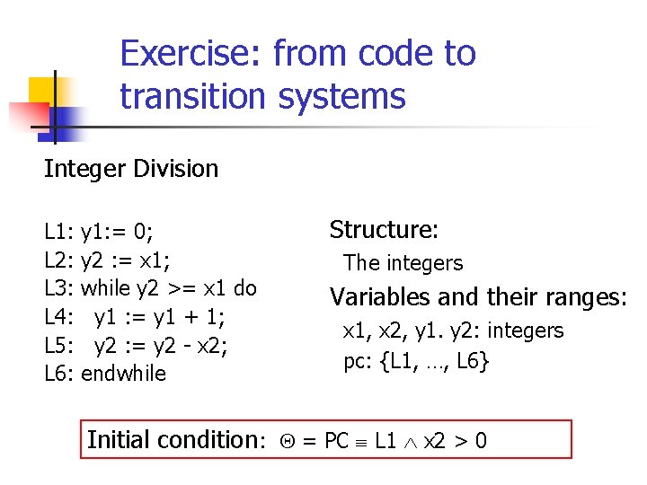
Exercise: from code to transition systems Integer Division L 1: L 2: L 3: L 4: L 5: L 6: y 1: = 0; y 2 : = x 1; while y 2 >= x 1 do y 1 : = y 1 + 1; y 2 : = y 2 - x 2; endwhile Structure: The integers Variables and their ranges: x 1, x 2, y 1. y 2: integers pc: {L 1, …, L 6} Initial condition: = PC L 1 x 2 > 0

Exercise: from code to transition systems Transitions:

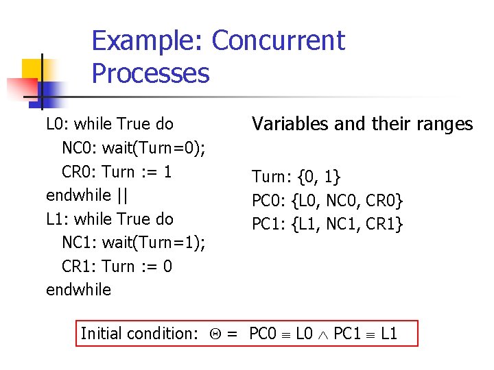
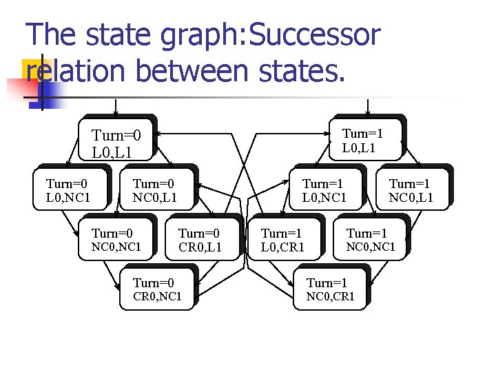
Example: Concurrent Processes L 0: while True do NC 0: wait(Turn=0); CR 0: Turn : = 1 endwhile || L 1: while True do NC 1: wait(Turn=1); CR 1: Turn : = 0 endwhile Variables and their ranges Turn: {0, 1} PC 0: {L 0, NC 0, CR 0} PC 1: {L 1, NC 1, CR 1} Initial condition: = PC 0 L 0 PC 1 L 1

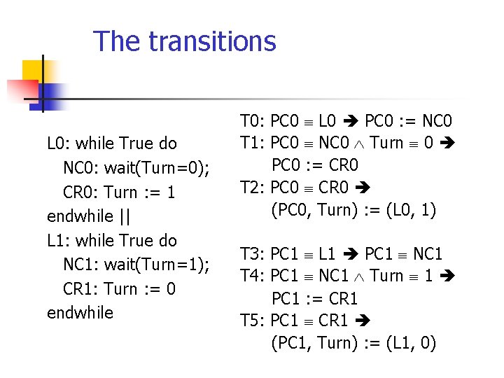
The transitions L 0: while True do NC 0: wait(Turn=0); CR 0: Turn : = 1 endwhile || L 1: while True do NC 1: wait(Turn=1); CR 1: Turn : = 0 endwhile T 0: PC 0 L 0 PC 0 : = NC 0 T 1: PC 0 NC 0 Turn 0 PC 0 : = CR 0 T 2: PC 0 CR 0 (PC 0, Turn) : = (L 0, 1) T 3: PC 1 L 1 PC 1 NC 1 T 4: PC 1 NC 1 Turn 1 PC 1 : = CR 1 T 5: PC 1 CR 1 (PC 1, Turn) : = (L 1, 0)

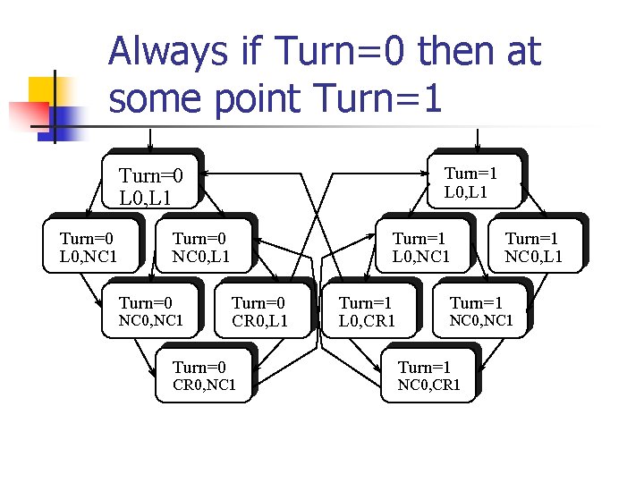
The state graph: Successor relation between states. Turn=1 L 0, L 1 Turn=0 L 0, NC 1 Turn=0 NC 0, L 1 Turn=0 NC 0, NC 1 Turn=0 Turn=1 L 0, NC 1 Turn=0 CR 0, L 1 CR 0, NC 1 Turn=1 L 0, CR 1 Turn=1 NC 0, L 1 NC 0, NC 1 Turn=1 NC 0, CR 1

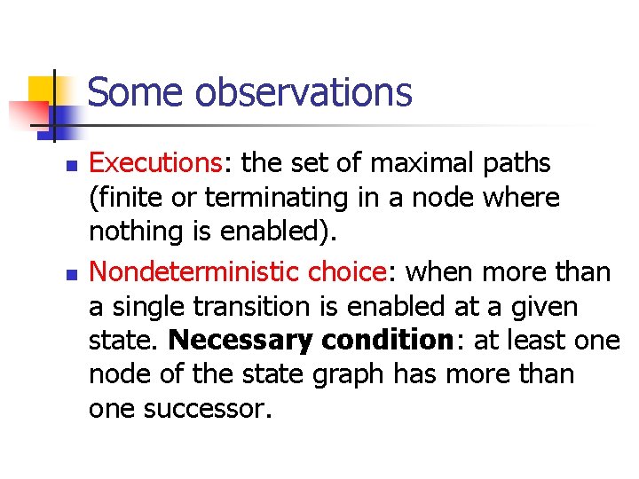
Some observations n n Executions: the set of maximal paths (finite or terminating in a node where nothing is enabled). Nondeterministic choice: when more than a single transition is enabled at a given state. Necessary condition: at least one node of the state graph has more than one successor.

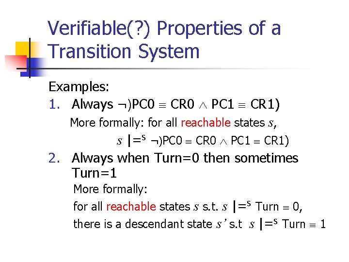
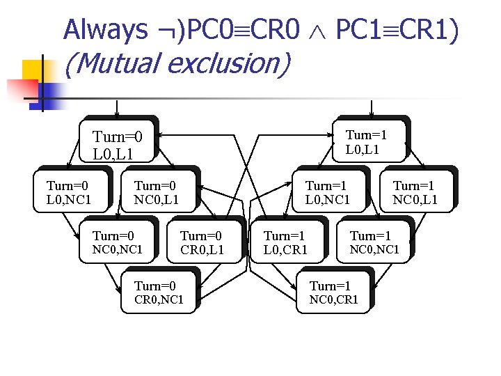
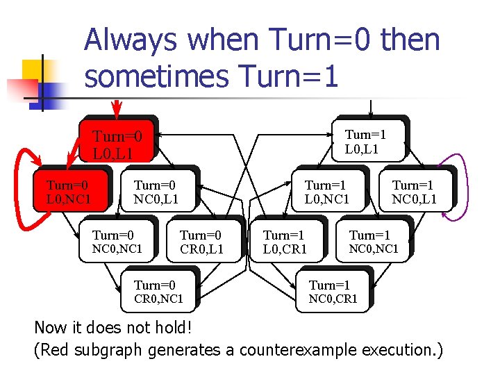
Verifiable(? ) Properties of a Transition System Examples: 1. Always ¬)PC 0 CR 0 PC 1 CR 1) More formally: for all reachable states s, s |=S ¬)PC 0 CR 0 PC 1 CR 1) 2. Always when Turn=0 then sometimes Turn=1 More formally: for all reachable states s s. t. s |=S Turn 0, there is a descendant state s’ s. t s |=S Turn 1

Always ¬)PC 0 CR 0 PC 1 CR 1) (Mutual exclusion) Turn=1 L 0, L 1 Turn=0 L 0, NC 1 Turn=0 NC 0, L 1 Turn=0 NC 0, NC 1 Turn=0 Turn=1 L 0, NC 1 Turn=0 CR 0, L 1 CR 0, NC 1 Turn=1 L 0, CR 1 Turn=1 NC 0, L 1 NC 0, NC 1 Turn=1 NC 0, CR 1

Always if Turn=0 then at some point Turn=1 L 0, L 1 Turn=0 L 0, NC 1 Turn=0 NC 0, L 1 Turn=0 NC 0, NC 1 Turn=0 Turn=1 L 0, NC 1 Turn=0 CR 0, L 1 CR 0, NC 1 Turn=1 L 0, CR 1 Turn=1 NC 0, L 1 NC 0, NC 1 Turn=1 NC 0, CR 1

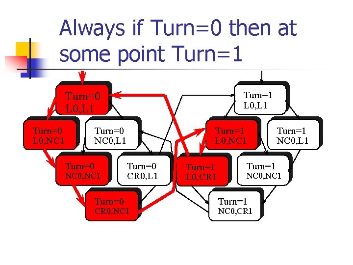
Always if Turn=0 then at some point Turn=1 L 0, L 1 Turn=0 L 0, NC 1 Turn=0 NC 0, L 1 Turn=0 NC 0, NC 1 Turn=0 Turn=1 L 0, NC 1 Turn=0 CR 0, L 1 CR 0, NC 1 Turn=1 L 0, CR 1 Turn=1 NC 0, L 1 NC 0, NC 1 Turn=1 NC 0, CR 1

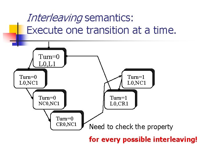
Interleaving semantics: Execute one transition at a time. Turn=0 L 0, L 1 Turn=0 L 0, NC 1 Turn=1 L 0, NC 1 Turn=0 NC 0, NC 1 Turn=1 L 0, CR 1 Turn=0 CR 0, NC 1 Need to check the property for every possible interleaving!

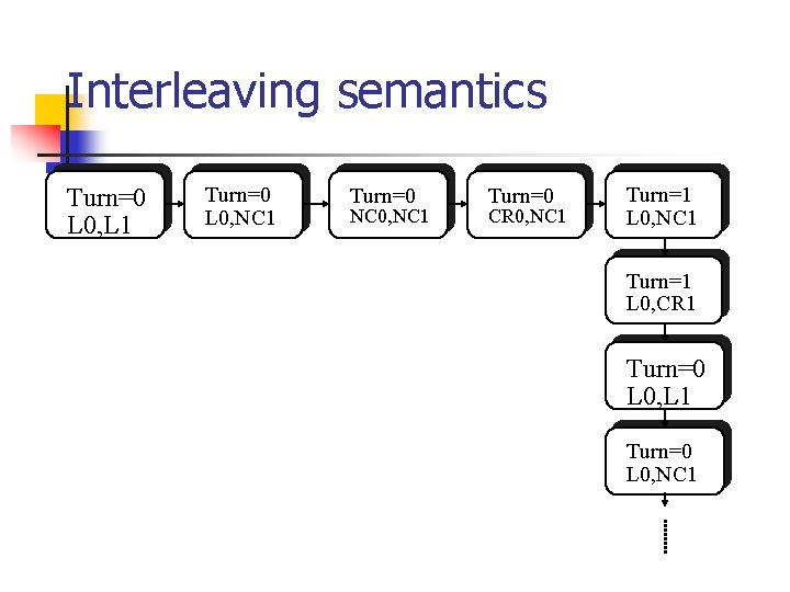
Interleaving semantics Turn=0 L 0, L 1 Turn=0 L 0, NC 1 Turn=0 NC 0, NC 1 Turn=0 CR 0, NC 1 Turn=1 L 0, CR 1 Turn=0 L 0, L 1 Turn=0 L 0, NC 1

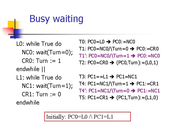
Busy waiting L 0: while True do NC 0: wait(Turn=0); CR 0: Turn : = 1 endwhile || L 1: while True do NC 1: wait(Turn=1); CR 1: Turn : = 0 endwhile T 0: PC 0=L 0 PC 0: =NC 0 T 1: PC 0=NC 0/Turn=0 PC 0: =CR 0 T 1’: PC 0=NC 0/Turn=1 PC 0: =NC 0 T 2: PC 0=CR 0 (PC 0, Turn): =(L 0, 1) T 3: PC 1==L 1 PC 1=NC 1 T 4: PC 1=NC 1/Turn=1 PC 1: =CR 1 T 4’: PC 1=NC 1/Turn=0 PC 1: =NC 1 T 5: PC 1=CR 1 (PC 1, Turn): =(L 1, 0) Initially: PC 0=L 0 / PC 1=L 1

Always when Turn=0 then sometimes Turn=1 L 0, L 1 Turn=0 L 0, NC 1 Turn=0 NC 0, L 1 Turn=0 NC 0, NC 1 Turn=0 Turn=1 L 0, NC 1 Turn=0 CR 0, L 1 CR 0, NC 1 Turn=1 L 0, CR 1 Turn=1 NC 0, L 1 Turn=1 NC 0, NC 1 Turn=1 NC 0, CR 1 Now it does not hold! (Red subgraph generates a counterexample execution. )

Combining Systems

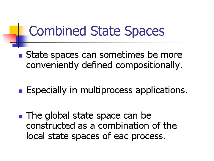
Combined State Spaces n n n State spaces can sometimes be more conveniently defined compositionally. Especially in multiprocess applications. The global state space can be constructed as a combination of the local state spaces of eac process.

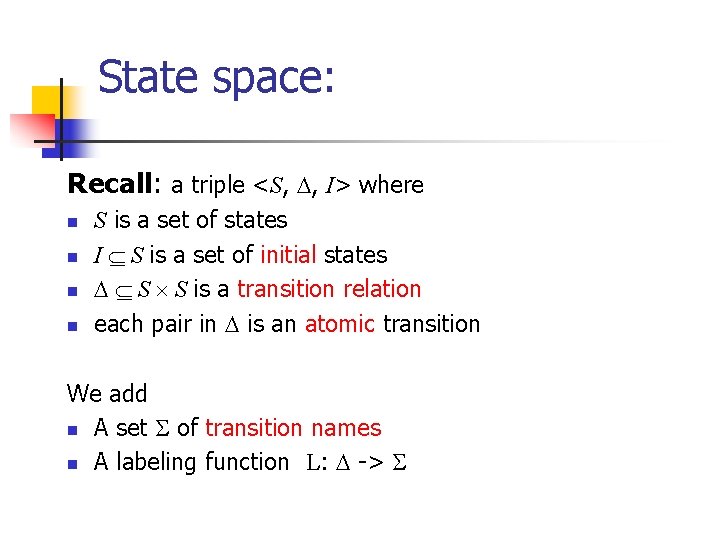
State space: Recall: a triple <S, , I> where n n S is a set of states I S is a set of initial states S S is a transition relation each pair in is an atomic transition We add n A set of transition names n A labeling function L: ->

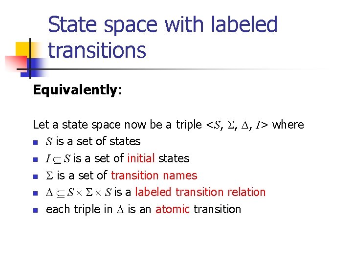
State space with labeled transitions Equivalently: Let a state space now be a triple <S, , , I> where n S is a set of states n I S is a set of initial states n is a set of transition names n S S is a labeled transition relation n each triple in is an atomic transition

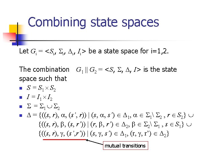
Combining state spaces Let Gi = <Si, i, Ii> be a state space for i=1, 2. The combination G 1 || G 2 = <S, , , I> is the state space such that n S = S 1 S 2 n I = I 1 I 2 n = 1 2 n = {((s, r), , (s’, r)) | (s, , s’) 1, 1 2 , r S 2} {((s, r), , (s, r’)) | (r, , r’) 2, 2 1 , s S 1} {((s, r), , (s’, r’)) | (s, , s’) 1, (r, , r’) 2} mutual transitions

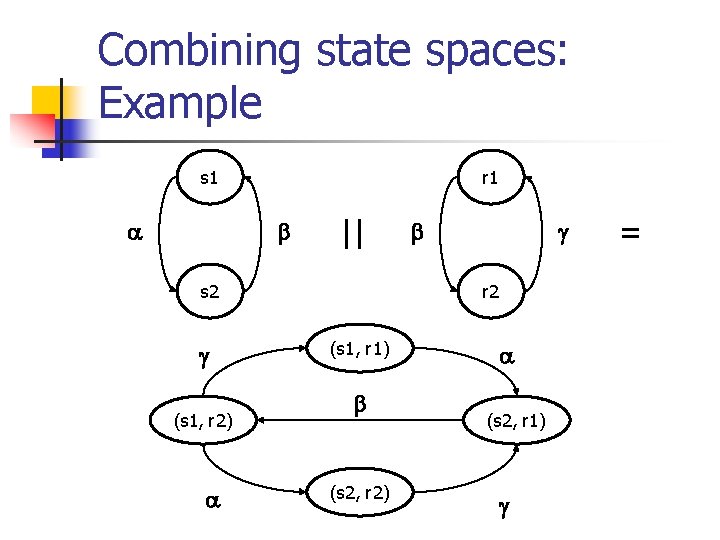
Combining state spaces: Example s 1 r 1 || s 2 (s 1, r 2) r 2 (s 1, r 1) (s 2, r 2) (s 2, r 1) =

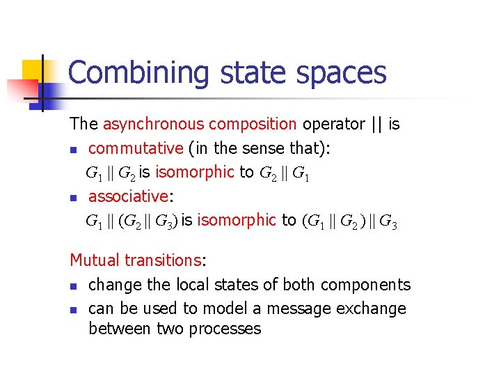
Combining state spaces The asynchronous composition operator || is n commutative (in the sense that): G 1 || G 2 is isomorphic to G 2 || G 1 n associative: G 1 || (G 2 || G 3) is isomorphic to (G 1 || G 2 ) || G 3 Mutual transitions: n change the local states of both components n can be used to model a message exchange between two processes

Fairness

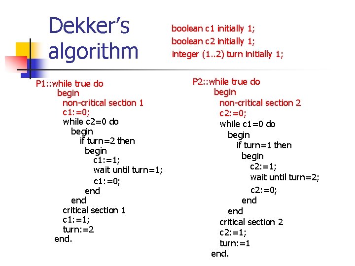
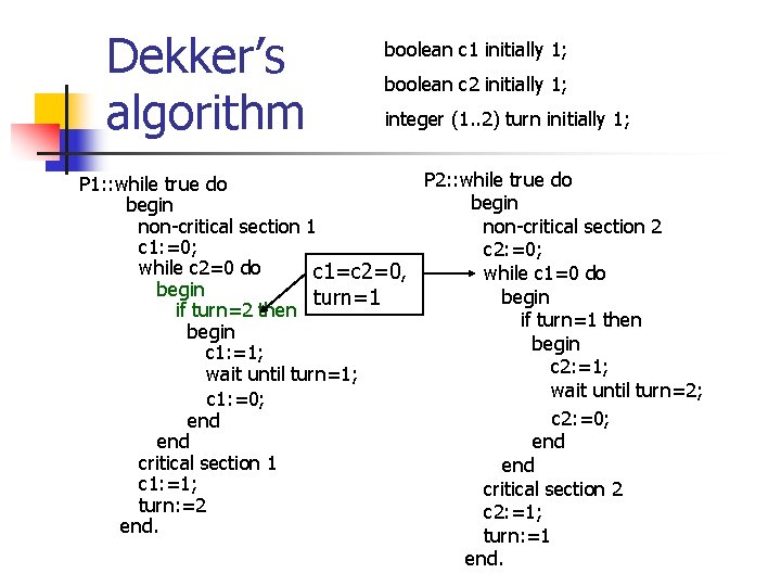
Dekker’s algorithm P 1: : while true do begin non-critical section 1 c 1: =0; while c 2=0 do begin if turn=2 then begin c 1: =1; wait until turn=1; c 1: =0; end critical section 1 c 1: =1; turn: =2 end. boolean c 1 initially 1; boolean c 2 initially 1; integer (1. . 2) turn initially 1; P 2: : while true do begin non-critical section 2 c 2: =0; while c 1=0 do begin if turn=1 then begin c 2: =1; wait until turn=2; c 2: =0; end critical section 2 c 2: =1; turn: =1 end.

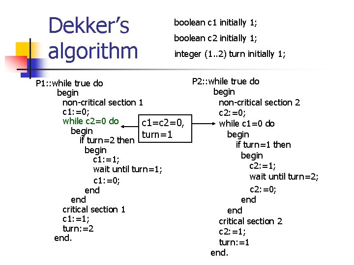
Dekker’s algorithm boolean c 1 initially 1; boolean c 2 initially 1; integer (1. . 2) turn initially 1; P 2: : while true do P 1: : while true do begin non-critical section 1 non-critical section 2 c 1: =0; c 2: =0; while c 2=0 do c 1=c 2=0, while c 1=0 do begin turn=1 if turn=2 then if turn=1 then begin c 1: =1; c 2: =1; wait until turn=2; c 1: =0; c 2: =0; end end critical section 1 end c 1: =1; critical section 2 turn: =2 c 2: =1; end. turn: =1 end.

Dekker’s algorithm boolean c 1 initially 1; boolean c 2 initially 1; integer (1. . 2) turn initially 1; P 2: : while true do P 1: : while true do begin non-critical section 1 non-critical section 2 c 1: =0; c 2: =0; while c 2=0 do c 1=c 2=0, while c 1=0 do begin turn=1 if turn=2 then if turn=1 then begin c 1: =1; c 2: =1; wait until turn=2; c 1: =0; c 2: =0; end end critical section 1 end c 1: =1; critical section 2 turn: =2 c 2: =1; end. turn: =1 end.

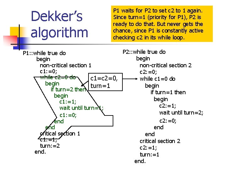
Dekker’s algorithm P 1 waits for P 2 to set c 2 to 1 again. Since turn=1 (priority for P 1), P 2 is ready to do that. But never gets the chance, since P 1 is constantly active checking c 2 in its while loop. P 2: : while true do P 1: : while true do begin non-critical section 1 non-critical section 2 c 1: =0; c 2: =0; while c 2=0 do c 1=c 2=0, while c 1=0 do begin turn=1 if turn=2 then if turn=1 then begin c 1: =1; c 2: =1; wait until turn=2; c 1: =0; c 2: =0; end end critical section 1 end c 1: =1; critical section 2 turn: =2 c 2: =1; end. turn: =1 end.

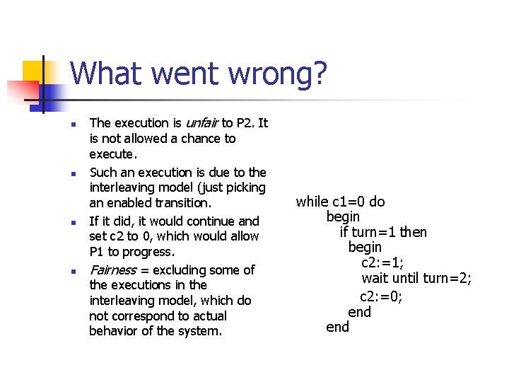
What went wrong? n n The execution is unfair to P 2. It is not allowed a chance to execute. Such an execution is due to the interleaving model (just picking an enabled transition. If it did, it would continue and set c 2 to 0, which would allow P 1 to progress. Fairness = excluding some of the executions in the interleaving model, which do not correspond to actual behavior of the system. while c 1=0 do begin if turn=1 then begin c 2: =1; wait until turn=2; c 2: =0; end

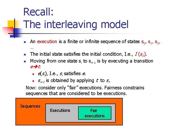
Recall: The interleaving model n n n An execution is a finite or infinite sequence of states s 0, s 1, s 2, … The initial state satisfies the initial condition, I. e. , I (s 0). Moving from one state si to si+1 is by executing a transition e t: n e(si), I. e. , si satisfies e. n si+1 is obtained by applying t to si. Now: consider only “fair” executions. Fairness constrains sequences that are considered to be executions. Sequences Executions Fair executions

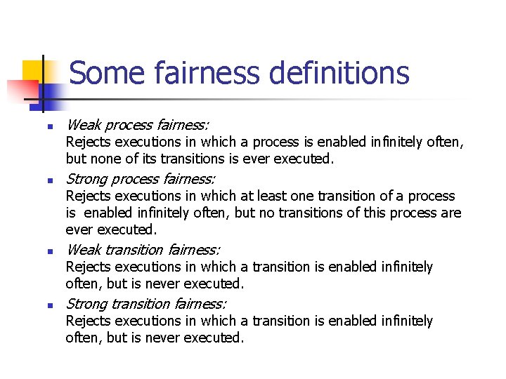
Some fairness definitions n Weak process fairness: Rejects executions in which a process is enabled infinitely often, but none of its transitions is ever executed. n Strong process fairness: Rejects executions in which at least one transition of a process is enabled infinitely often, but no transitions of this process are ever executed. n Weak transition fairness: Rejects executions in which a transition is enabled infinitely often, but is never executed. n Strong transition fairness: Rejects executions in which a transition is enabled infinitely often, but is never executed.

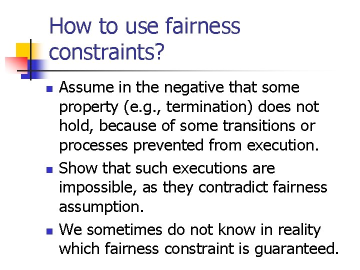
How to use fairness constraints? n n n Assume in the negative that some property (e. g. , termination) does not hold, because of some transitions or processes prevented from execution. Show that such executions are impossible, as they contradict fairness assumption. We sometimes do not know in reality which fairness constraint is guaranteed.

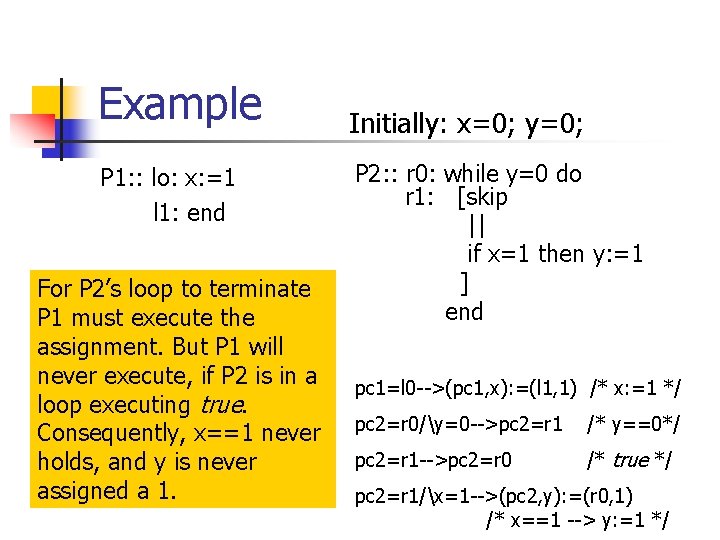
Example P 1: : lo: x: =1 l 1: end For P 2’s loop to terminate P 1 must execute the assignment. But P 1 will never execute, if P 2 is in a loop executing true. Consequently, x==1 never holds, and y is never assigned a 1. Initially: x=0; y=0; P 2: : r 0: while y=0 do r 1: [skip || if x=1 then y: =1 ] end pc 1=l 0 -->(pc 1, x): =(l 1, 1) /* x: =1 */ pc 2=r 0/y=0 -->pc 2=r 1 /* y==0*/ pc 2=r 1 -->pc 2=r 0 /* true */ pc 2=r 1/x=1 -->(pc 2, y): =(r 0, 1) /* x==1 --> y: =1 */

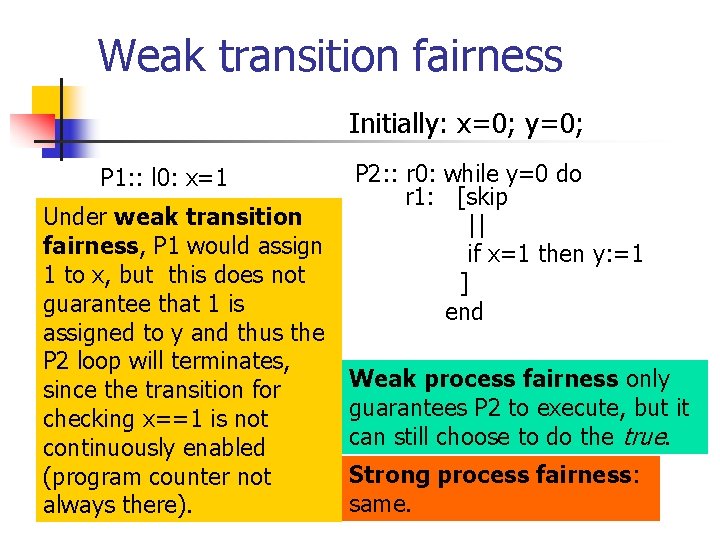
Weak transition fairness Initially: x=0; y=0; P 1: : l 0: x=1 Under weak transition fairness, P 1 would assign 1 to x, but this does not guarantee that 1 is assigned to y and thus the P 2 loop will terminates, since the transition for checking x==1 is not continuously enabled (program counter not always there). P 2: : r 0: while y=0 do r 1: [skip || if x=1 then y: =1 ] end Weak process fairness only guarantees P 2 to execute, but it can still choose to do the true. Strong process fairness: same.

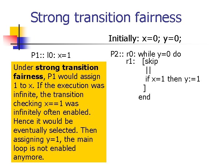
Strong transition fairness Initially: x=0; y=0; P 2: : r 0: while y=0 do r 1: [skip Under strong transition || fairness, P 1 would assign if x=1 then y: =1 1 to x. If the execution was ] infinite, the transition end checking x==1 was infinitely often enabled. Hence it would be eventually selected. Then assigning y=1, the main loop is not enabled anymore. P 1: : l 0: x=1

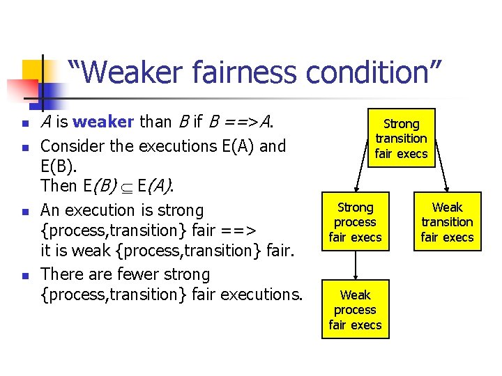
“Weaker fairness condition” n n A is weaker than B if B ==>A. Consider the executions E(A) and E(B). Then E(B) E(A). An execution is strong {process, transition} fair ==> it is weak {process, transition} fair. There are fewer strong {process, transition} fair executions. Strong transition fair execs Strong process fair execs Weak transition fair execs