The Topology of Wireless Communication Merav Parter Department

The Topology of Wireless Communication Merav Parter Department of Computer Science and Applied Mathematics Weizmann Institute Joint work with Erez Kantor, Zvi Lotker and David Peleg WRAWN Reykjavik, Iceland July 2011

Goal Study Topological Properties of Reception Maps and their applications to Algorithmic Design

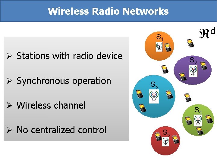
Wireless Radio Networks d S 1 Ø Stations with radio device Ø Synchronous operation S 2 S 3 Ø Wireless channel Ø No centralized control S 4 S 5

Physical Models Attempting to model attenuation and interference explicitly Most commonly used: Signal to Interference plus Noise Ratio (SINR)

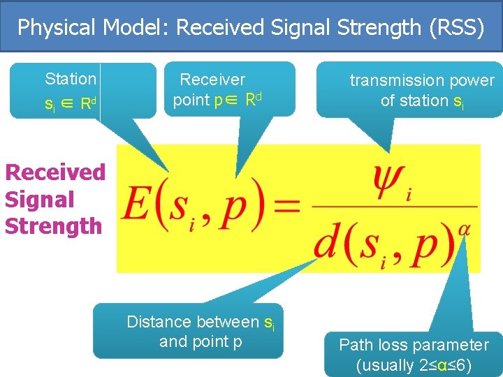
Physical Model: Received Signal Strength (RSS) Station si ∈ Rd Receiver point p∈ Rd transmission power of station si Received Signal Strength Distance between si and point p Path loss parameter (usually 2≤α≤ 6)

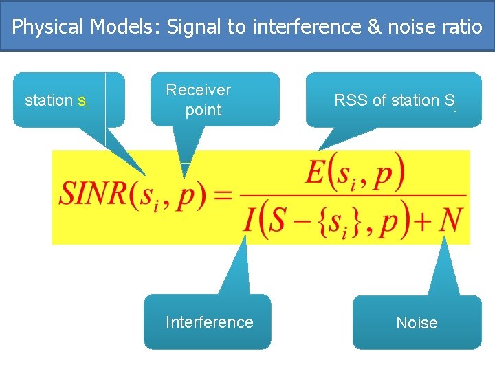
Physical Model: interference Interfering stations in Rd Receiver point RSS of station sj

Physical Models: Signal to interference & noise ratio station si Receiver point Interference RSS of station Sj Noise

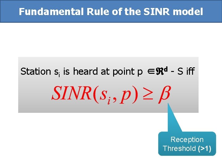
Fundamental Rule of the SINR model Station si is heard at point p ∈ d - S iff Reception Threshold (>1)

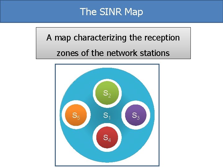
The SINR Map A map characterizing the reception zones of the network stations S 2 S 5 S 1 S 4 S 3

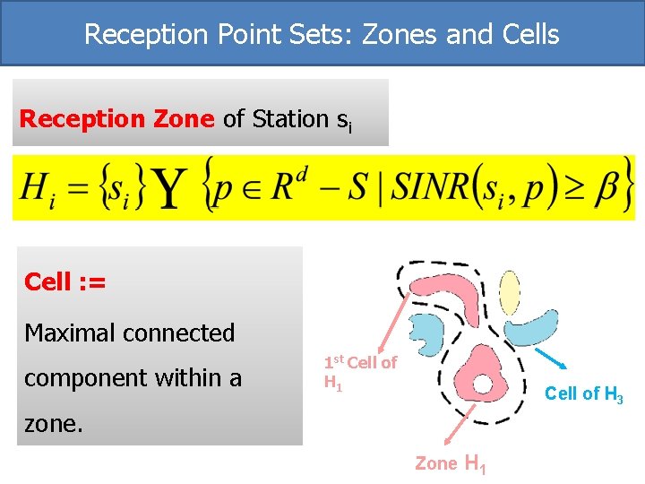
Reception Point Sets: Zones and Cells Reception Zone of Station si Cell : = Maximal connected component within a 1 st Cell of H 1 Cell of H 3 zone. Zone H 1

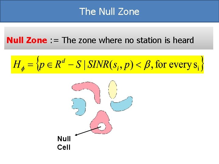
The Null Zone : = The zone where no station is heard Null Cell

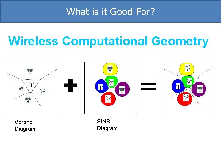
What is it Good For? Wireless Computational Geometry Voronoi Diagram SINR Diagram

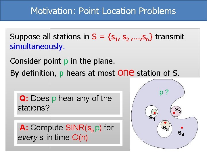
Motivation: Point Location Problems Suppose all stations in S = {s 1, s 2 , …, sn} transmit simultaneously. Consider point p in the plane. By definition, p hears at most one station of S. p? Q: Does p hear any of the stations? s 2 s 1 A: Compute SINR(si, p) for every si in time O(n) s 3 s 4

Algorithmic Question s 1 s 2 s 3 Can we answer point location queries FASTER? s 4

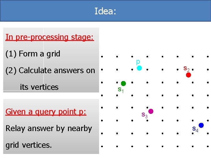
Idea: In pre-processing stage: (1) Form a grid p (2) Calculate answers on its vertices Given a query point p: Relay answer by nearby grid vertices. s 2 s 1 s 3 s 4

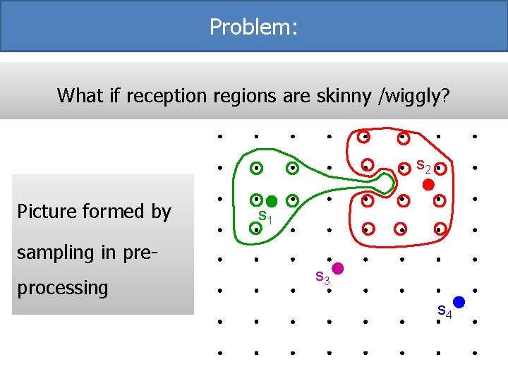
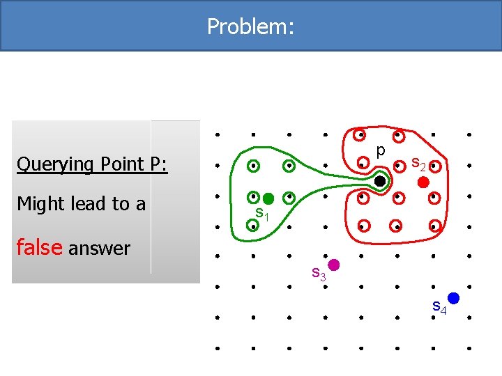
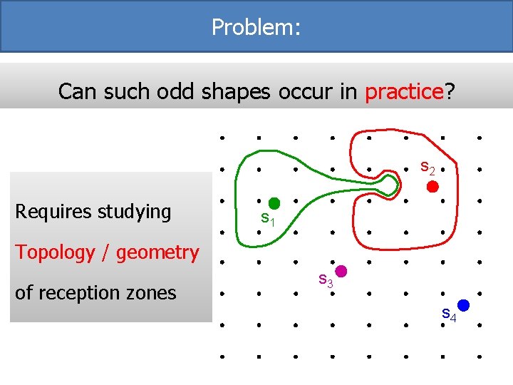
Problem: What if reception regions are skinny /wiggly? s 2 Picture formed by s 1 sampling in preprocessing s 3 s 4

Problem: p Querying Point P: Might lead to a s 2 s 1 false answer s 3 s 4

Problem: Can such odd shapes occur in practice? s 2 Requires studying s 1 Topology / geometry of reception zones s 3 s 4

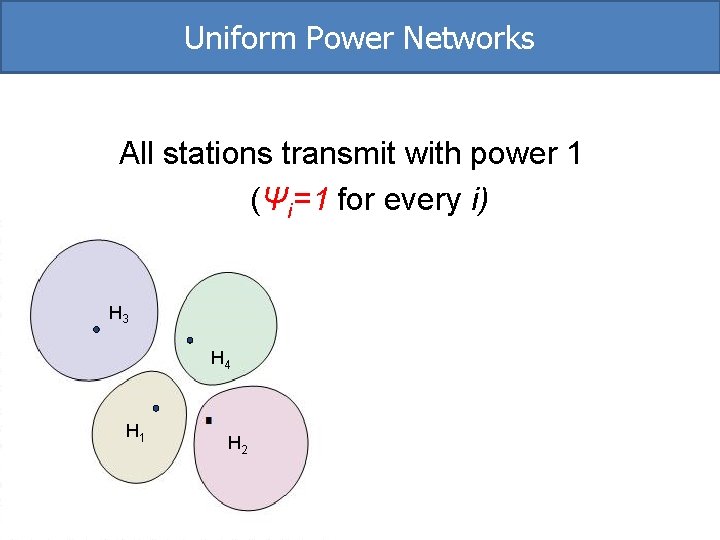
Uniform Power Networks All stations transmit with power 1 (Ψi=1 for every i) H 3 H 4 H 1 H 2

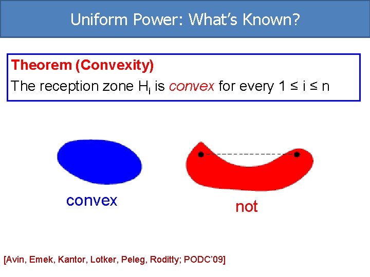
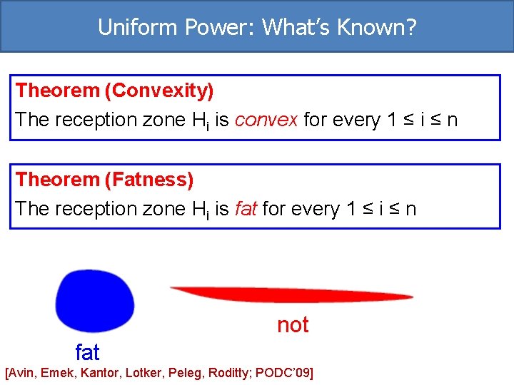
Uniform Power: What’s Known? Theorem (Convexity) The reception zone Hi is convex for every 1 ≤ i ≤ n convex [Avin, Emek, Kantor, Lotker, Peleg, Roditty; PODC’ 09] not

Uniform Power: What’s Known? Theorem (Convexity) The reception zone Hi is convex for every 1 ≤ i ≤ n Theorem (Fatness) The reception zone Hi is fat for every 1 ≤ i ≤ n not fat [Avin, Emek, Kantor, Lotker, Peleg, Roditty; PODC’ 09]

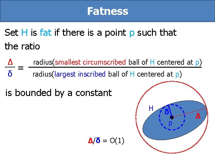
Fatness Set H is fat if there is a point p such that the ratio Δ radius(smallest circumscribed ball of H centered at p) = δ radius(largest inscribed ball of H centered at p) is bounded by a constant H δ p Δ/δ = O(1) Δ

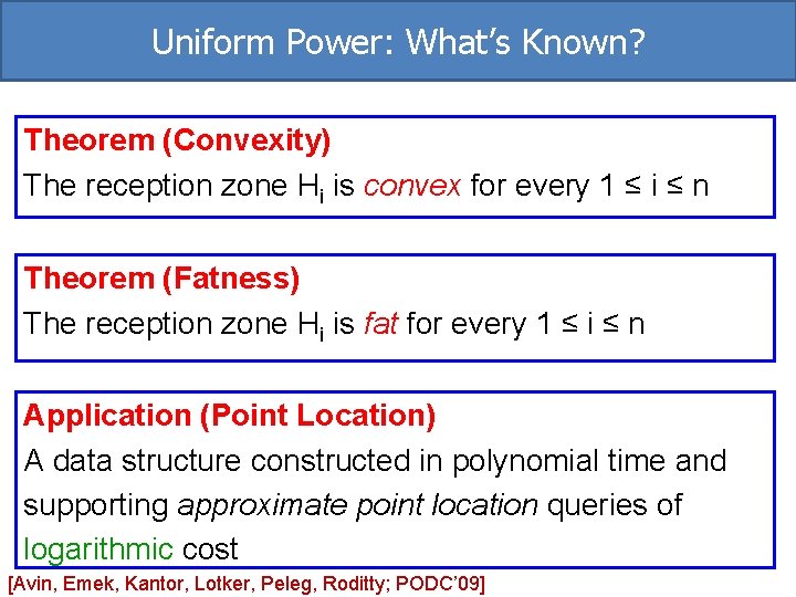
Uniform Power: What’s Known? Theorem (Convexity) The reception zone Hi is convex for every 1 ≤ i ≤ n Theorem (Fatness) The reception zone Hi is fat for every 1 ≤ i ≤ n Application (Point Location) A data structure constructed in polynomial time and supporting approximate point location queries of logarithmic cost [Avin, Emek, Kantor, Lotker, Peleg, Roditty; PODC’ 09]

Non-Uniform SINR Diagrams Stations may transmit with varying transmitting powers (different Ψi values) What are the fundamental properties of SINR maps for such networks?

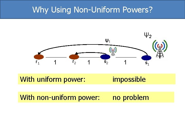
Why Using Non-Uniform Powers? ψ2 ψ1 r 1 1 r 2 1 s 1 With uniform power: impossible With non-uniform power: no problem

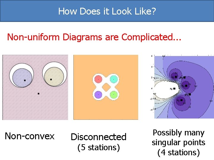
How Does it Look Like? Non-uniform Diagrams are Complicated. . . Non-convex Disconnected (5 stations) Possibly many singular points (4 stations)

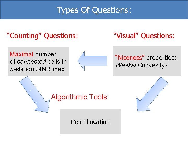
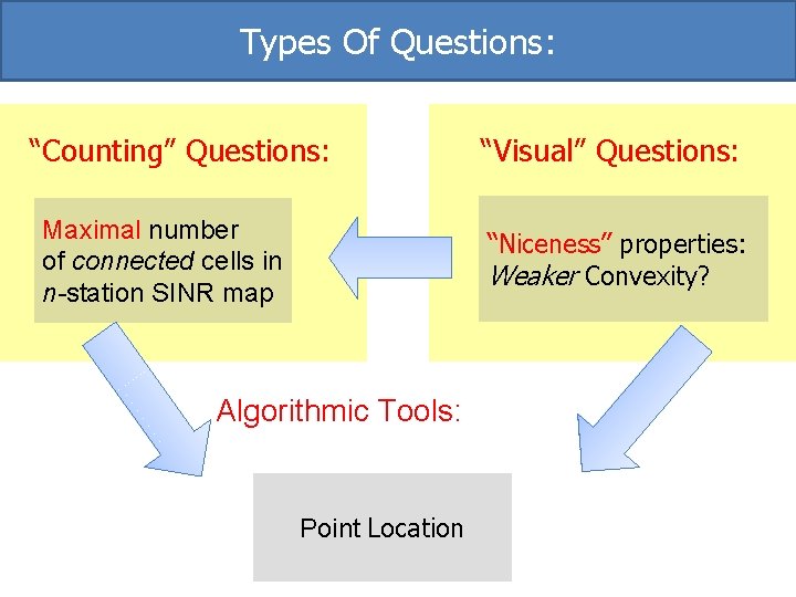
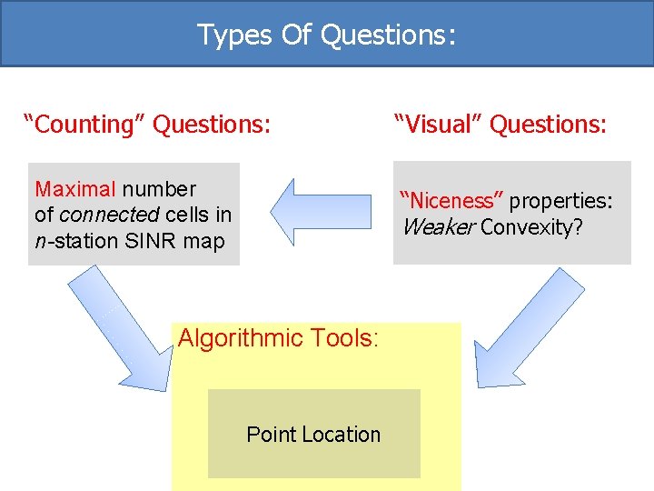
Types Of Questions: “Counting” Questions: Maximal number of connected cells in n-station SINR map “Visual” Questions: “Niceness” properties: Weaker Convexity? Algorithmic Tools: Point Location

SINR Map & Voronoi Diagram

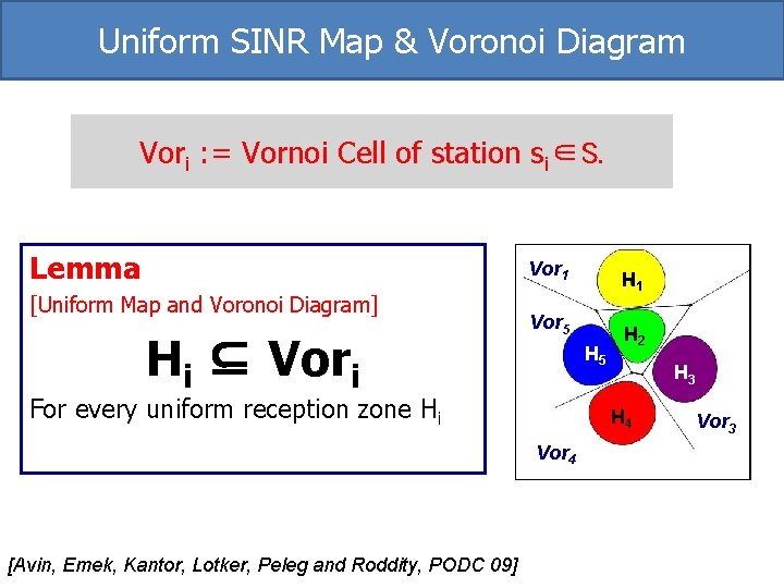
Uniform SINR Map & Voronoi Diagram Vori : = Vornoi Cell of station si∈S. Lemma [Uniform Map and Voronoi Diagram] Hi ⊆ Vori Vor 1 H 11 H Vor 5 H 22 H HH 55 For every uniform reception zone Hi H 44 H Vor 4 [Avin, Emek, Kantor, Lotker, Peleg and Roddity, PODC 09] H 33 H Vor 3

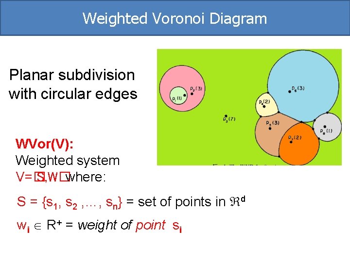
Weighted Voronoi Diagram Planar subdivision with circular edges WVor(V): Weighted system V=� S, W�where: S = {s 1, s 2 , …, sn} = set of points in d wi R+ = weight of point si

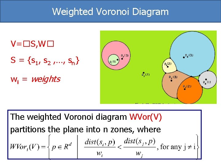
Weighted Voronoi Diagram V=�S, W� S = {s 1, s 2 , …, sn} wi = weights The weighted Voronoi diagram WVor(V) partitions the plane into n zones, where

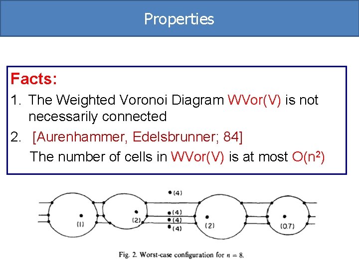
Properties Facts: 1. The Weighted Voronoi Diagram WVor(V) is not necessarily connected 2. [Aurenhammer, Edelsbrunner; 84] The number of cells in WVor(V) is at most O(n 2)

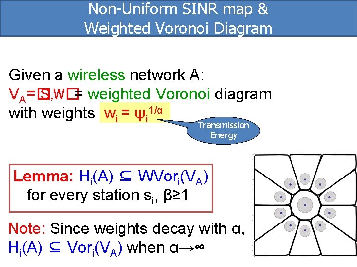
Non-Uniform SINR map & Weighted Voronoi Diagram Given a wireless network A: VA=� S, W�= weighted Voronoi diagram with weights wi = ψi 1/α Transmission Energy Lemma: Hi(A) ⊆ WVori(VA) for every station si, β≥ 1 Note: Since weights decay with α, Hi(A) ⊆ Vori(VA) when α→∞

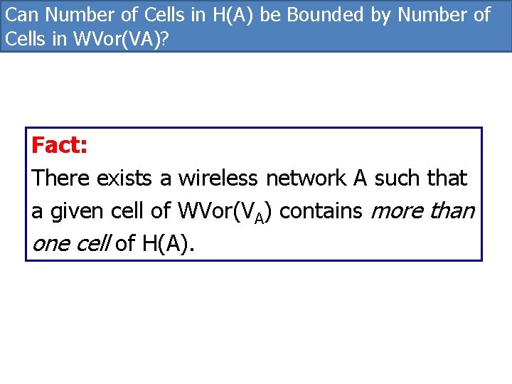
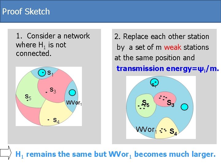
Can Number of Cells in H(A) be Bounded by Number of Cells in WVor(VA)? Fact: There exists a wireless network A such that a given cell of WVor(VA) contains more than one cell of H(A).

Proof Sketch 1. Consider a network where H 1 is not connected. s 1 s 5 2. Replace each other station by a set of m weak stations at the same position and transmission energy=ψi/m. s 1 s 3 WVor 1 S 5 S 3 s 4 WVor 1 S 4 H 1 remains the same but WVor 1 becomes much larger.

Types Of Questions: “Counting” Questions: Maximal number of connected cells in n-station SINR map “Visual” Questions: “Niceness” properties: Weaker Convexity? Algorithmic Tools: Point Location

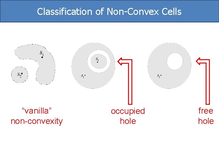
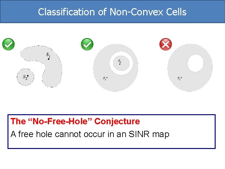
Classification of Non-Convex Cells “vanilla” non-convexity occupied hole free hole

Classification of Non-Convex Cells The “No-Free-Hole” Conjecture A free hole cannot occur in an SINR map

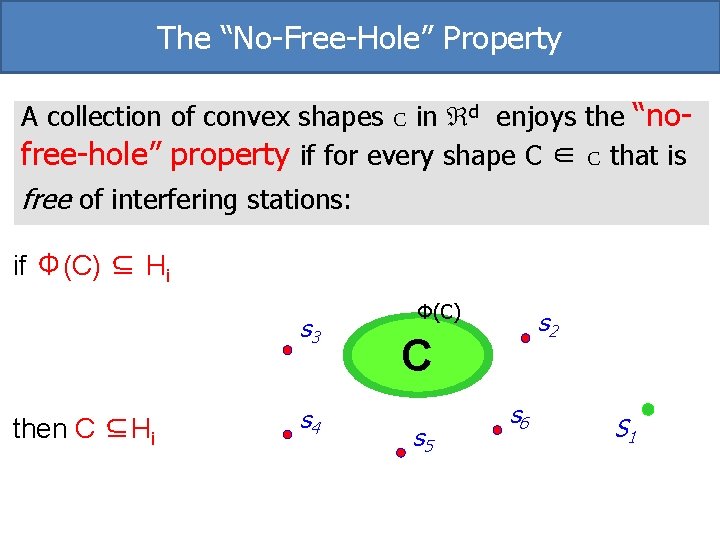
The “No-Free-Hole” Property A collection of convex shapes C in d enjoys the “nofree-hole” property if for every shape C ∈ C that is free of interfering stations: if Φ(C) ⊆ Hi s 3 then C ⊆Hi s 4 Φ(C) s 2 C s 5 s 6 S 1

The Big Question Do SINR zones satisfy the “no-free-hole” property ?

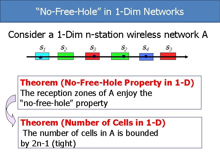
“No-Free-Hole” in 1 -Dim Networks Consider a 1 -Dim n-station wireless network A s 1 s 2 s 3 s 2 s 4 s 3 Theorem (No-Free-Hole Property in 1 -D) The reception zones of A enjoy the “no-free-hole” property Theorem (Number of Cells in 1 -D) The number of cells in A is bounded by 2 n-1 (tight)

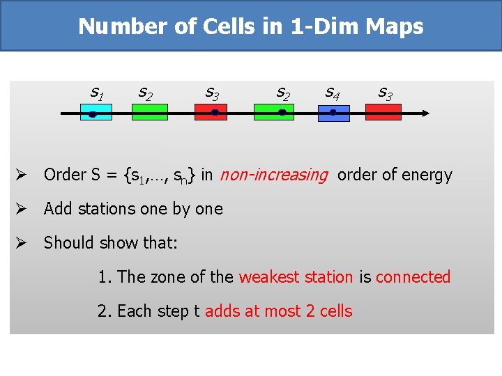
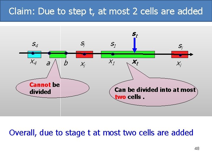
Number of Cells in 1 -Dim Maps s 1 s 2 s 3 s 2 s 4 s 3 Ø Order S = {s 1, …, sn} in non-increasing order of energy Ø Add stations one by one Ø Should show that: 1. The zone of the weakest station is connected 2. Each step t adds at most 2 cells

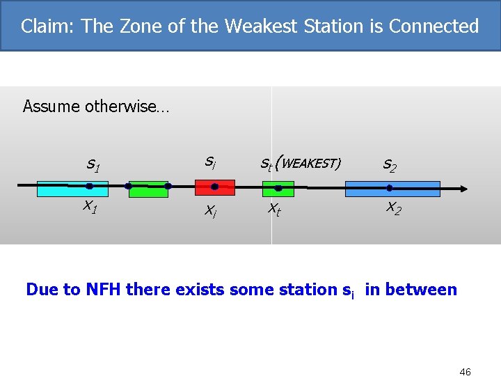
Claim: The Zone of the Weakest Station is Connected Assume otherwise… s 1 si x 1 xi st (WEAKEST) xt s 2 x 2 Due to NFH there exists some station si in between 46

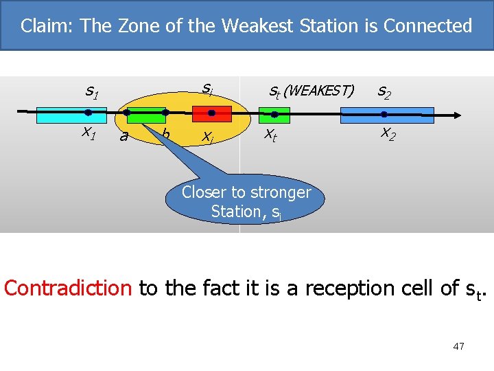
Claim: The Zone of the Weakest Station is Connected s 1 x 1 a b si st (WEAKEST) s 2 xi xt x 2 Closer to stronger Station, si Contradiction to the fact it is a reception cell of st. 47

Claim: Due to step t, at most 2 cells are added s 4 x 4 a Cannot be divided b si s 1 xi x 1 st si xt xi Can be divided into at most two cells. Overall, due to stage t at most two cells are added 48

“No-Free-Hole” Property in d? Conjecture: For a d-dimensional n-station network A, the reception zones of H(A) enjoy the “no-free-hole” property in d

Bounding #Cells in Higher Dimensions Gap: The number of cells in an SINR map for d-Dim n-station wireless network is at most O(nd+1) and at least Ω(n)

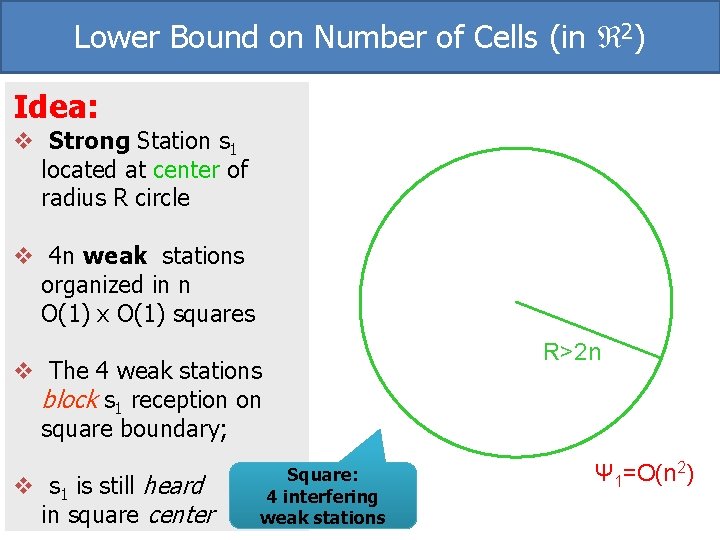
Lower Bound on Number of Cells (in 2 -Dim) Theorem: There exist 2 -Dim n-station wireless networks where s 1 has Ω(n) cells

Lower Bound on Number of Cells (in 2) Idea: v Strong Station s 1 located at center of radius R circle v 4 n weak stations organized in n O(1) x O(1) squares v The 4 weak stations block s 1 reception on square boundary; v s 1 is still heard in square center Square: 4 interfering weak stations R>2 n Ψ 1=O(n 2)

Connectivity & Convexity in Higher Dimensions

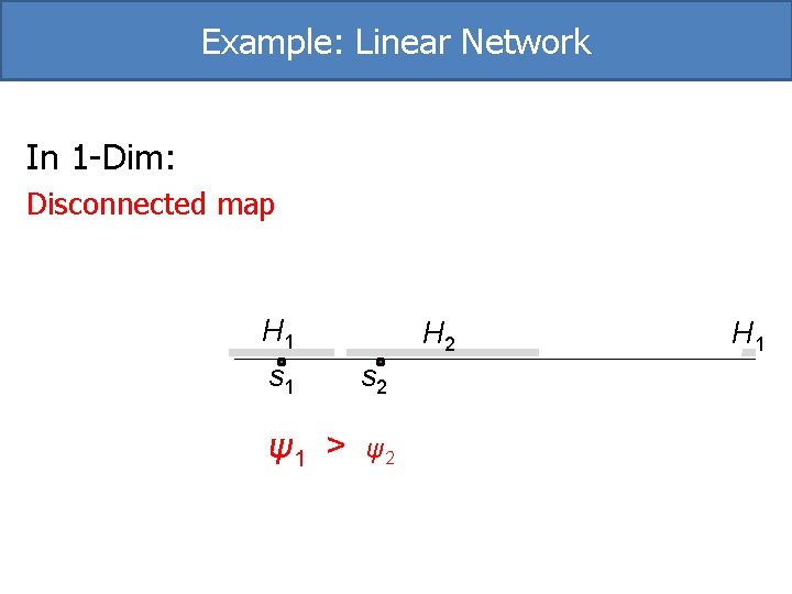
Example: Linear Network In 1 -Dim: Disconnected map H 1 s 2 ψ1 > ψ2 H 1

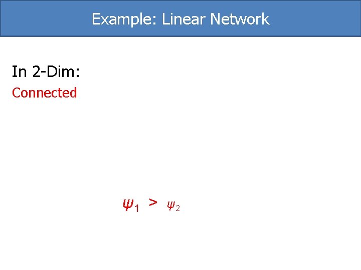
Example: Linear Network In 2 -Dim: Connected ψ1 > ψ2

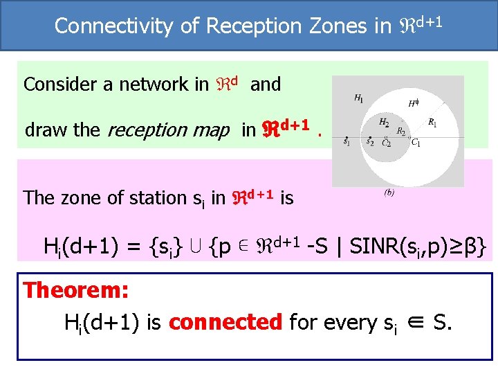
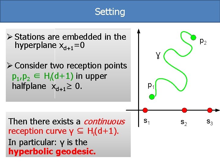
Connectivity of Reception Zones in d+1 Consider a network in d and draw the reception map in d+1. The zone of station si in d+1 is Hi(d+1) = {si} ⋃ {p ∊ d+1 -S | SINR(si, p)≥β} Theorem: Hi(d+1) is connected for every si ∈ S.

Setting Ø Stations are embedded in the hyperplane xd+1=0 Ø Consider two reception points p 1, p 2 ∈ Hi(d+1) in upper halfplane xd+1≥ 0. Then there exists a continuous reception curve γ ⊆ Hi(d+1). In particular: γ is the hyperbolic geodesic. p 2 Ɣ p 1 s 2 s 3

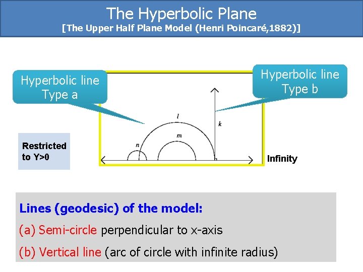
The Hyperbolic Plane [The Upper Half Plane Model (Henri Poincaré, 1882)] Hyperbolic line Type a Restricted to Y>0 Hyperbolic line Type b Infinity Lines (geodesic) of the model: (a) Semi-circle perpendicular to x-axis (b) Vertical line (arc of circle with infinite radius)

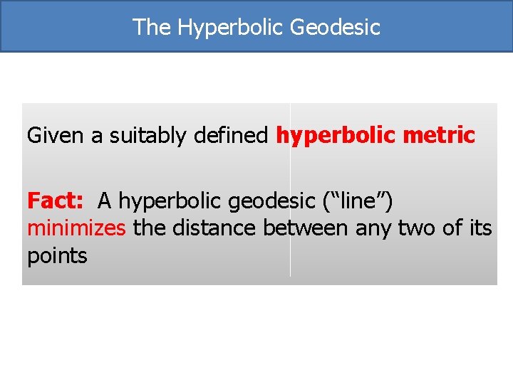
The Hyperbolic Geodesic Given a suitably defined hyperbolic metric Fact: A hyperbolic geodesic (“line”) minimizes the distance between any two of its points

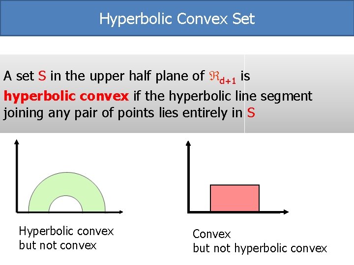
Hyperbolic Convex Set A set S in the upper half plane of d+1 is hyperbolic convex if the hyperbolic line segment joining any pair of points lies entirely in S Hyperbolic convex but not convex Convex but not hyperbolic convex

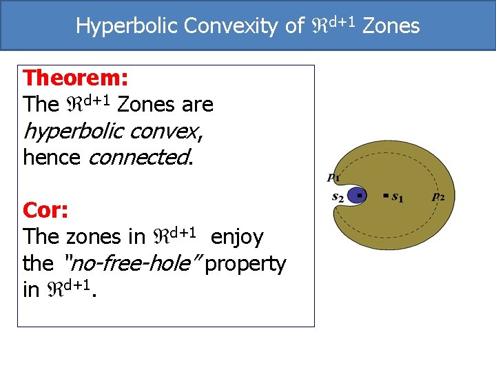
Hyperbolic Convexity of d+1 Zones Theorem: The d+1 Zones are hyperbolic convex, hence connected. Cor: The zones in d+1 enjoy the “no-free-hole” property in d+1.

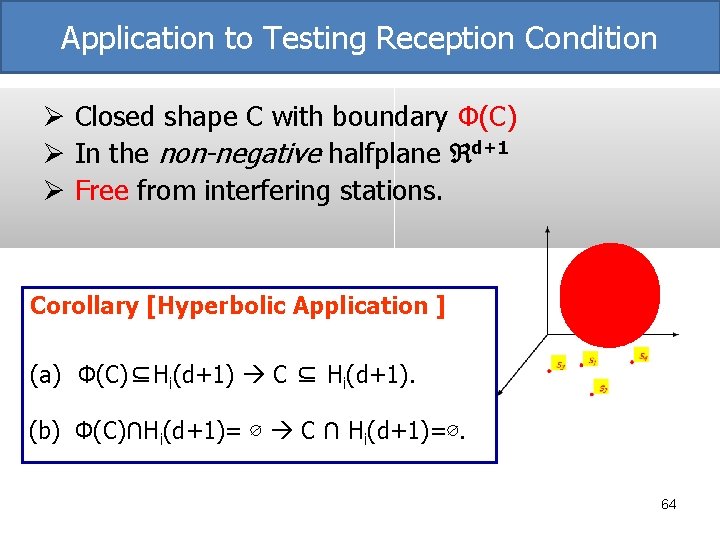
Application to Testing Reception Condition Ø Closed shape C with boundary Φ(C) Ø In the non-negative halfplane d+1 Ø Free from interfering stations. Corollary [Hyperbolic Application ] (a) Φ(C)⊆Hi(d+1) C ⊆ Hi(d+1). (b) Φ(C)∩Hi(d+1)= ∅ C ∩ Hi(d+1)=∅. 64

Types Of Questions: “Counting” Questions: Maximal number of connected cells in n-station SINR map “Visual” Questions: “Niceness” properties: Weaker Convexity? Algorithmic Tools: Point Location

Point Location in Non-Uniform Case Problems • No Voronoi diagram • No convexity • No fatness Solution • Use Weighted Voronoi diagram • Employ more delicate tagging & querying methods

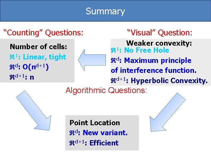
Summary “Counting” Questions: Number of cells: 1: Linear, tight d: O(nd+1) d+1: n “Visual” Question: Weaker convexity: 1: No Free Hole d: Maximum principle of interference function. d+1: Hyperbolic Convexity. Algorithmic Questions: Point Location d: New variant. d+1: Efficient

Thank You for Listening!