The Standard Normal Distribution Lesson 3 3 What

The Standard Normal Distribution Lesson 3. 3

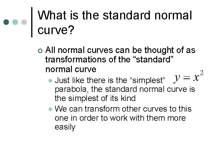
What is the standard normal curve? ¢ All normal curves can be thought of as transformations of the “standard” normal curve Just like there is the “simplest” parabola, the standard normal curve is the simplest of its kind l We can transform other curves to this one in order to work with them more easily l

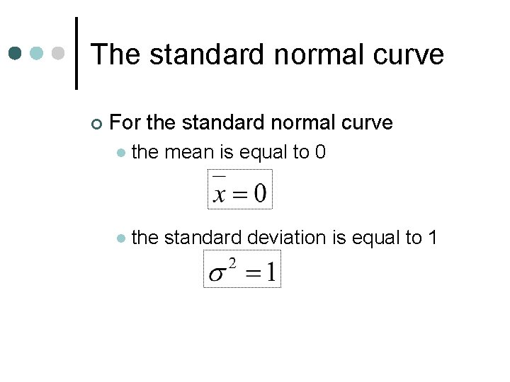
The standard normal curve ¢ For the standard normal curve l the mean is equal to 0 l the standard deviation is equal to 1

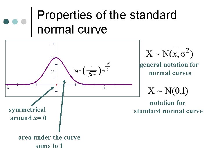
Properties of the standard normal curve general notation for normal curves symmetrical around x= 0 area under the curve sums to 1 notation for standard normal curve

Remember – this is Data EXAMPLE ¢ Imagine that you could tell how happy someone is by their “happiness score” A score of zero means you are at the “average” level of contentment l Positive scores mean that you are more happy l Negative scores mean that you are less happy l

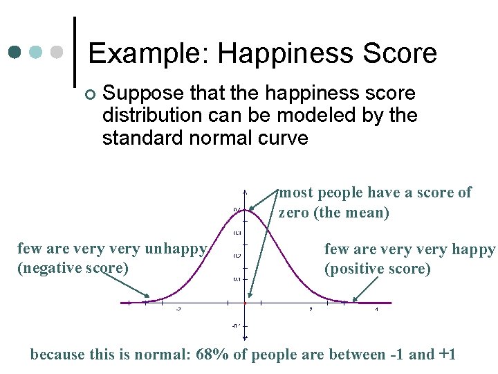
Example: Happiness Score ¢ Suppose that the happiness score distribution can be modeled by the standard normal curve most people have a score of zero (the mean) few are very unhappy (negative score) few are very happy (positive score) because this is normal: 68% of people are between -1 and +1

What’s so great about the standard normal curve? ¢ ¢ The x value is the same as the number of standard deviations away from the mean The area under the curve up to k is the same as the percent of data that has a value of k or less. The probability that x is less than P(x ≤ k) = Ak or equal to k is given by the area under the curve up to k

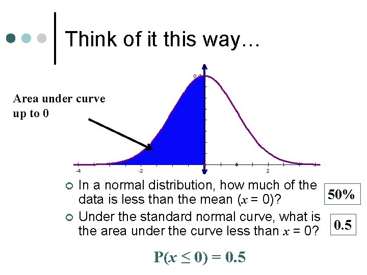
Think of it this way… Area under curve up to 0 ¢ ¢ In a normal distribution, how much of the 50% data is less than the mean (x = 0)? Under the standard normal curve, what is the area under the curve less than x = 0? 0. 5 P(x ≤ 0) = 0. 5

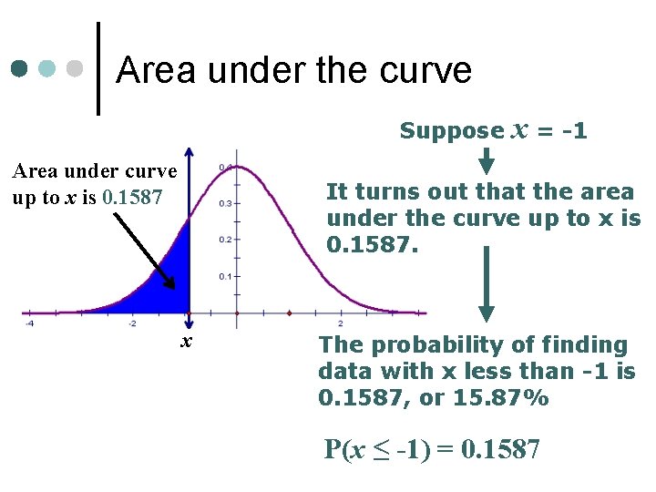
Area under the curve Suppose Area under curve up to x is 0. 1587 x = -1 It turns out that the area under the curve up to x is 0. 1587. x The probability of finding data with x less than -1 is 0. 1587, or 15. 87% P(x ≤ -1) = 0. 1587

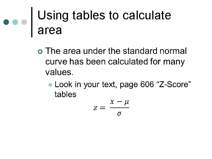
Using tables to calculate area ¢

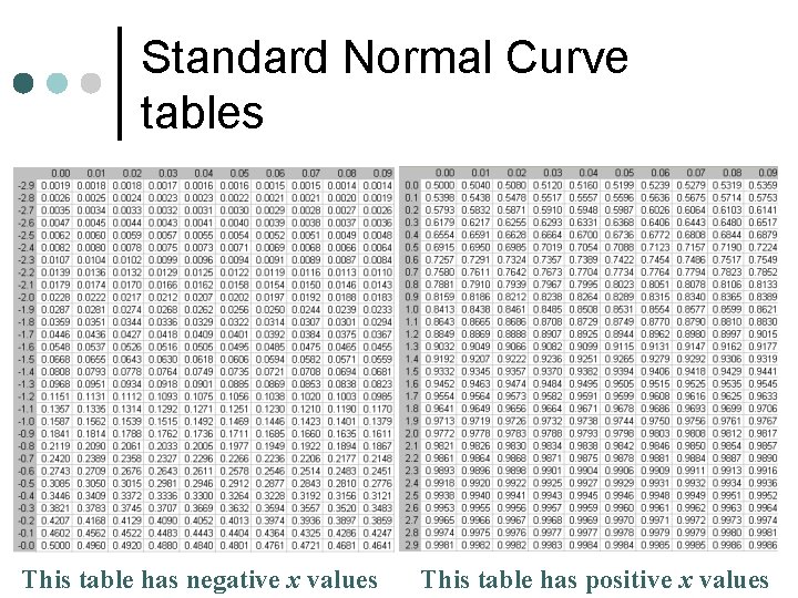
Standard Normal Curve tables This table has negative x values This table has positive x values

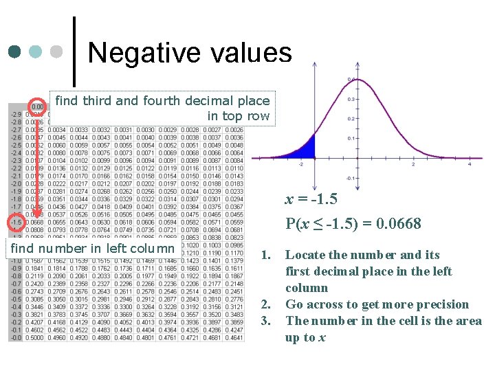
Negative values find third and fourth decimal place in top row x = -1. 5 P(x ≤ -1. 5) = 0. 0668 find number in left column 1. 2. 3. Locate the number and its first decimal place in the left column Go across to get more precision The number in the cell is the area up to x

Negative values x = -1. 85 P(x ≤ -1. 85) = 0. 0322 3. 22% of the data is less than or equal to -1. 85 This table has negative x values

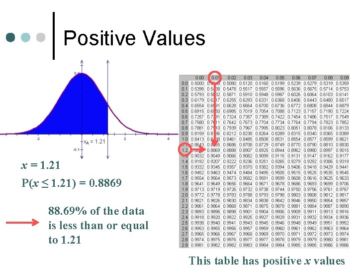
Positive Values x = 1. 21 P(x ≤ 1. 21) = 0. 8869 88. 69% of the data is less than or equal to 1. 21 This table has positive x values

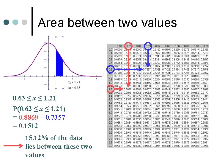
Area between two values 0. 63 ≤ x ≤ 1. 21 P(0. 63 ≤ x ≤ 1. 21) = 0. 8869 – 0. 7357 = 0. 1512 15. 12% of the data lies between these two values

See example 2 on page 426

See example 3 on page 428

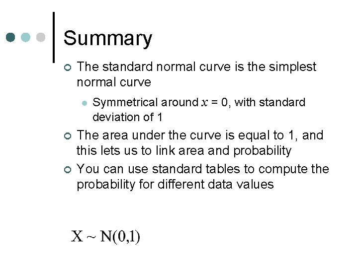
Summary ¢ The standard normal curve is the simplest normal curve l ¢ ¢ Symmetrical around x = 0, with standard deviation of 1 The area under the curve is equal to 1, and this lets us to link area and probability You can use standard tables to compute the probability for different data values

Practice: ¢ Page 430 #1 – 4, 6 -10