The Smoothed Analysis of Algorithms Simplex Methods and

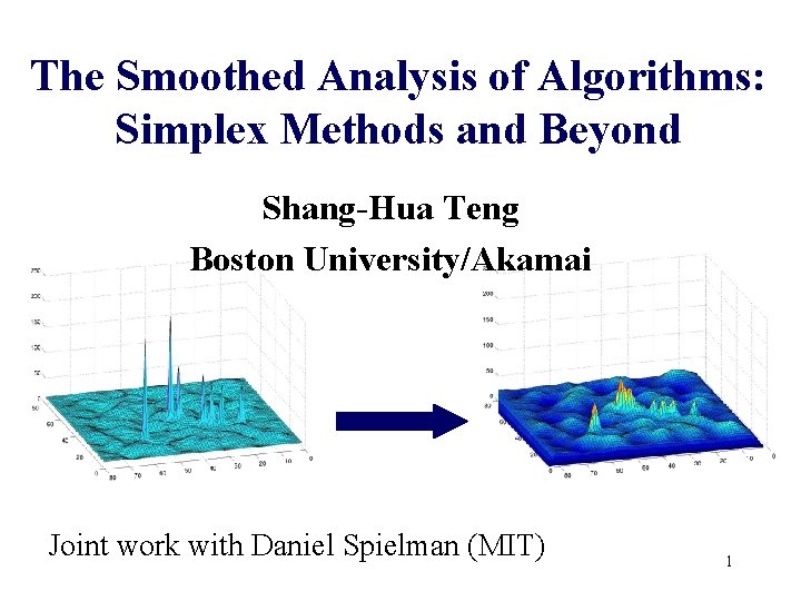
The Smoothed Analysis of Algorithms: Simplex Methods and Beyond Shang-Hua Teng Boston University/Akamai Joint work with Daniel Spielman (MIT) 1

Outline Why What Simplex Method Numerical Analysis Condition Numbers/Gaussian Elimination Conjectures and Open Problems 2

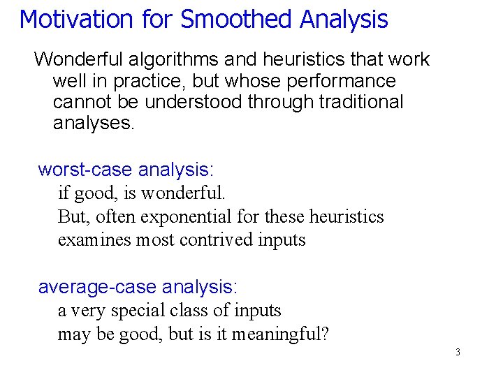
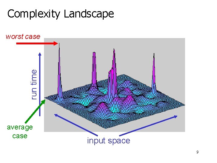
Motivation for Smoothed Analysis Wonderful algorithms and heuristics that work well in practice, but whose performance cannot be understood through traditional analyses. worst-case analysis: if good, is wonderful. But, often exponential for these heuristics examines most contrived inputs average-case analysis: a very special class of inputs may be good, but is it meaningful? 3

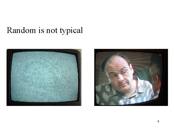
Random is not typical 4

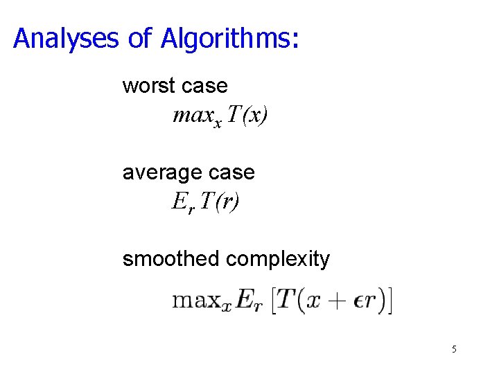
Analyses of Algorithms: worst case maxx T(x) average case Er T(r) smoothed complexity 5

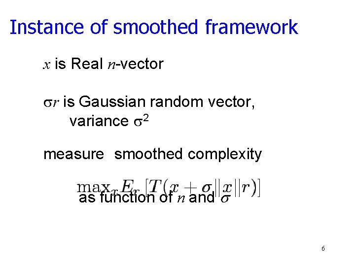
Instance of smoothed framework x is Real n-vector sr is Gaussian random vector, variance s 2 measure smoothed complexity as function of n and s 6

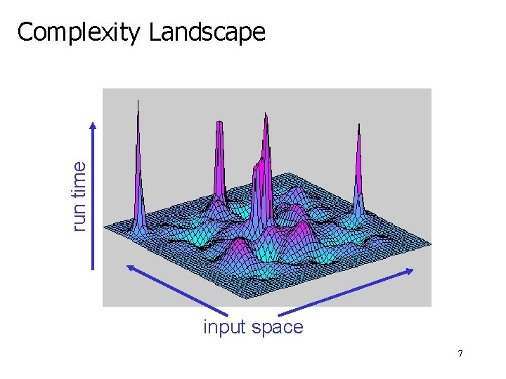
run time Complexity Landscape input space 7

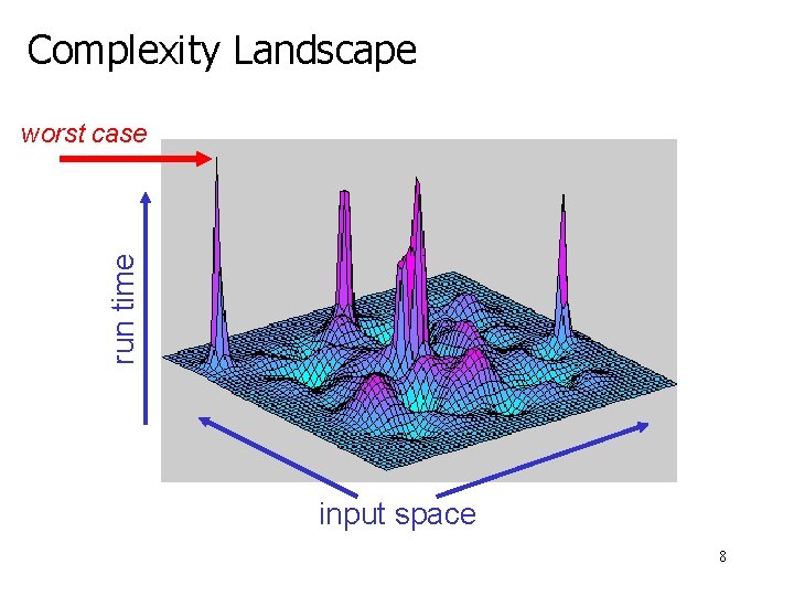
Complexity Landscape run time worst case input space 8

Complexity Landscape run time worst case average case input space 9

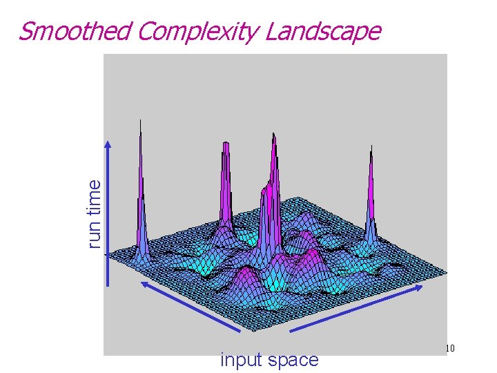
run time Smoothed Complexity Landscape input space 10

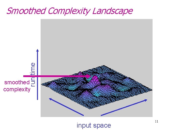
run time Smoothed Complexity Landscape smoothed complexity input space 11

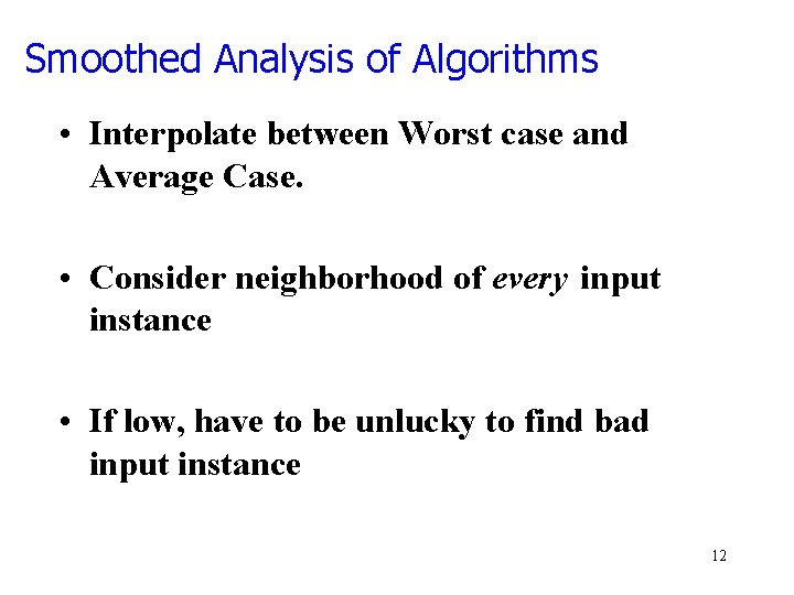
Smoothed Analysis of Algorithms • Interpolate between Worst case and Average Case. • Consider neighborhood of every input instance • If low, have to be unlucky to find bad input instance 12

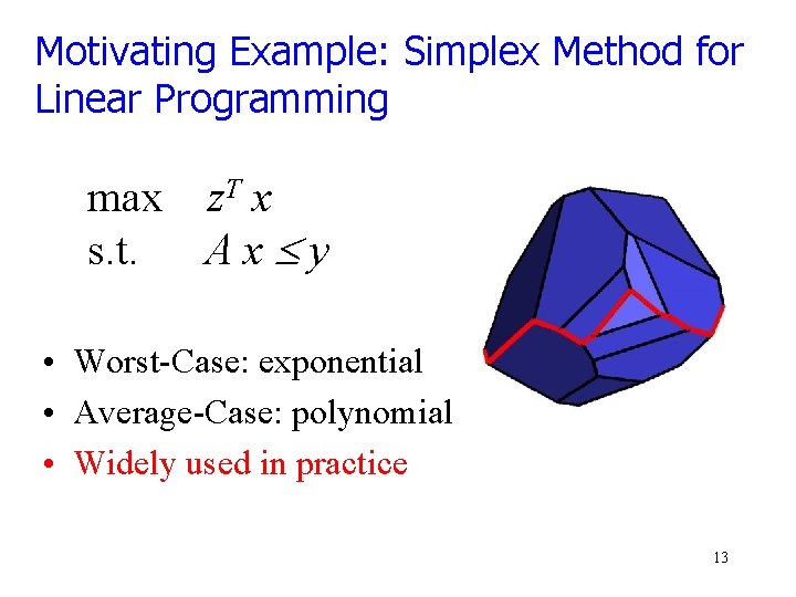
Motivating Example: Simplex Method for Linear Programming max z. T x s. t. Ax£y • Worst-Case: exponential • Average-Case: polynomial • Widely used in practice 13

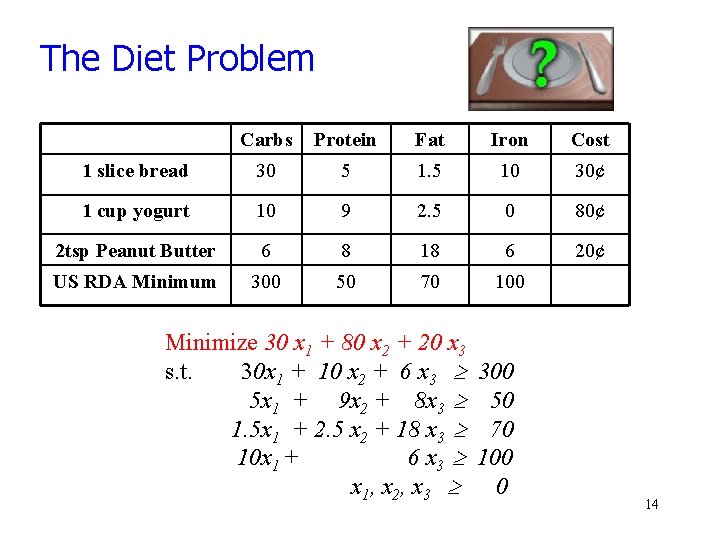
The Diet Problem Carbs Protein Fat Iron Cost 1 slice bread 30 5 10 30¢ 1 cup yogurt 10 9 2. 5 0 80¢ 2 tsp Peanut Butter 6 8 18 6 20¢ US RDA Minimum 300 50 70 100 Minimize 30 x 1 + 80 x 2 + 20 x 3 s. t. 30 x 1 + 10 x 2 + 6 x 3 5 x 1 + 9 x 2 + 8 x 3 1. 5 x 1 + 2. 5 x 2 + 18 x 3 10 x 1 + 6 x 3 x 1, x 2, x 3 300 50 70 100 0 14

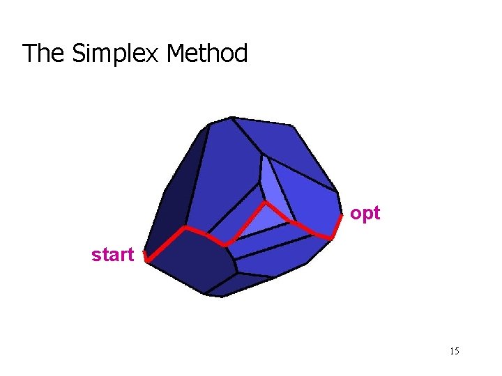
The Simplex Method opt start 15

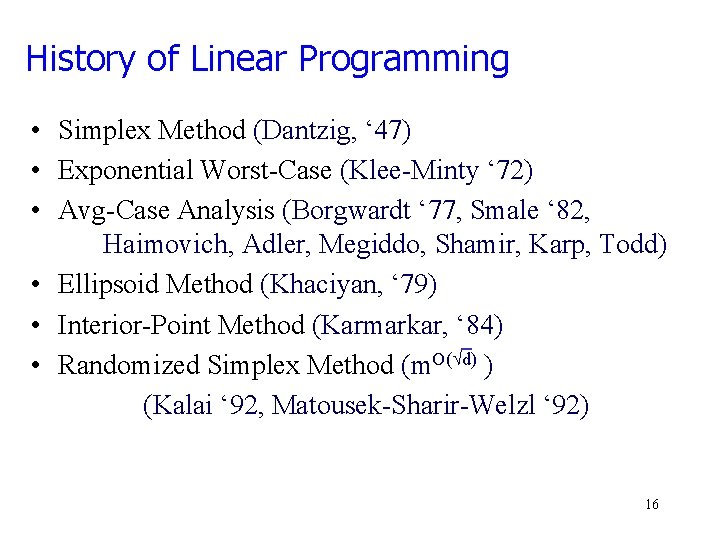
History of Linear Programming • Simplex Method (Dantzig, ‘ 47) • Exponential Worst-Case (Klee-Minty ‘ 72) • Avg-Case Analysis (Borgwardt ‘ 77, Smale ‘ 82, Haimovich, Adler, Megiddo, Shamir, Karp, Todd) • Ellipsoid Method (Khaciyan, ‘ 79) • Interior-Point Method (Karmarkar, ‘ 84) • Randomized Simplex Method (m. O( d) ) (Kalai ‘ 92, Matousek-Sharir-Welzl ‘ 92) 16

Smoothed Analysis of Simplex Method [Spielman-Teng 01] max z. T x s. t. Ax£y max s. t. z. T x G is Gaussian Theorem: For all A, simplex method takes expected time polynomial 17

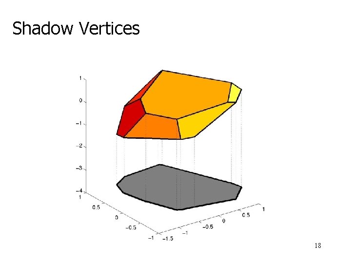
Shadow Vertices 18

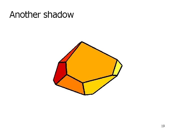
Another shadow 19

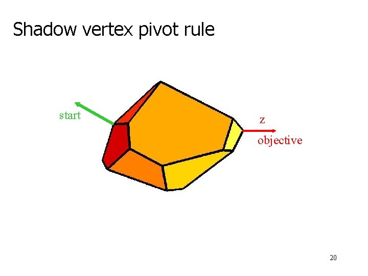
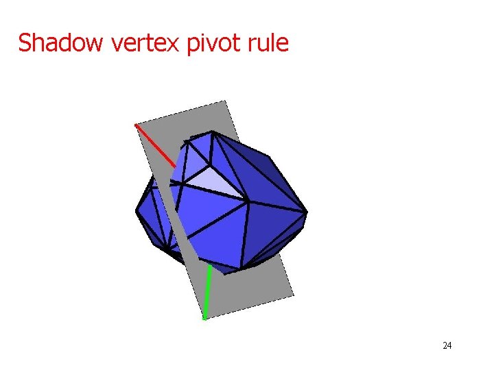
Shadow vertex pivot rule start z objective 20

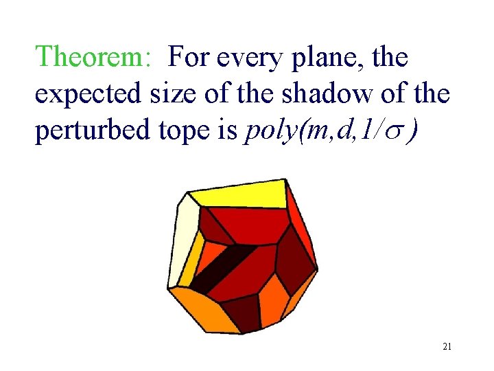
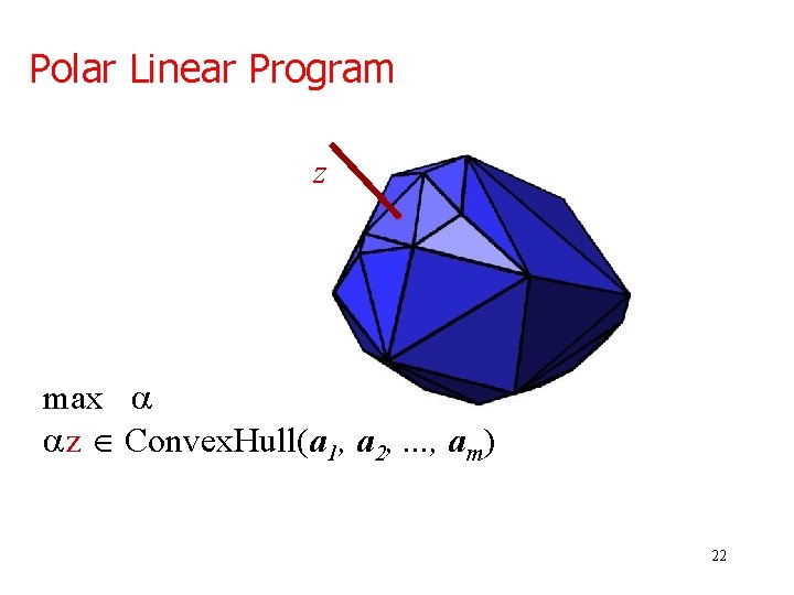
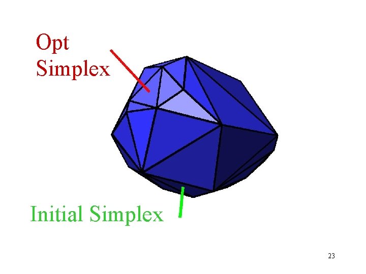
Theorem: For every plane, the expected size of the shadow of the perturbed tope is poly(m, d, 1/s ) 21

Polar Linear Program z max z Î Convex. Hull(a 1, a 2, . . . , am) 22

Opt Simplex Initial Simplex 23

Shadow vertex pivot rule 24

25

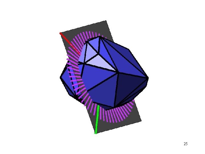
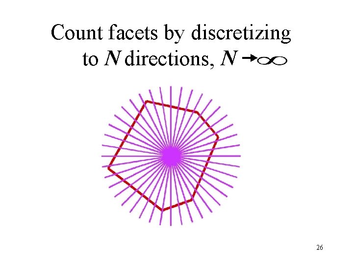
Count facets by discretizing to N directions, N 26

Count pairs in different facets Pr [ ] < c/N Different Facets So, expect c Facets 27

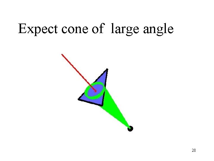
Expect cone of large angle 28

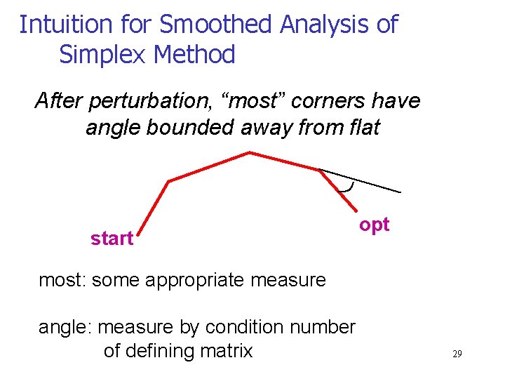
Intuition for Smoothed Analysis of Simplex Method After perturbation, “most” corners have angle bounded away from flat start opt most: some appropriate measure angle: measure by condition number of defining matrix 29

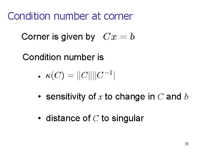
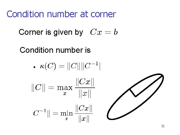
Condition number at corner Corner is given by Condition number is • • sensitivity of x to change in C and b • distance of C to singular 30

Condition number at corner Corner is given by Condition number is • 31

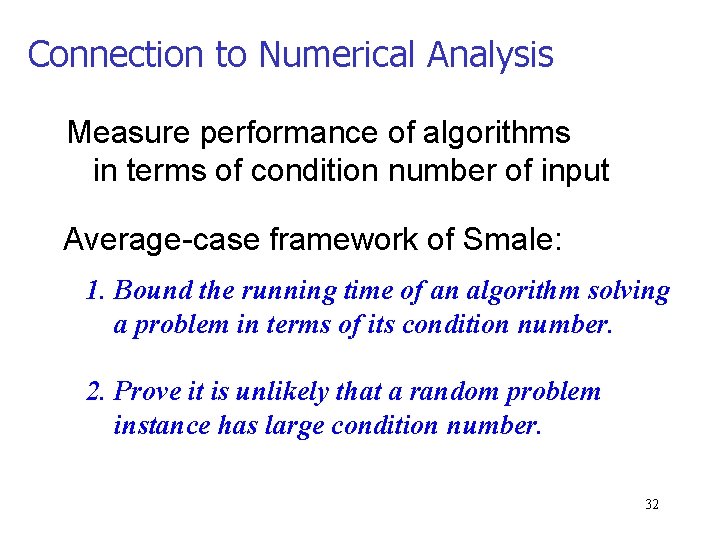
Connection to Numerical Analysis Measure performance of algorithms in terms of condition number of input Average-case framework of Smale: 1. Bound the running time of an algorithm solving a problem in terms of its condition number. 2. Prove it is unlikely that a random problem instance has large condition number. 32

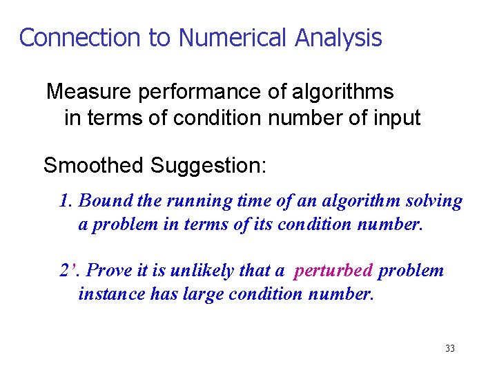
Connection to Numerical Analysis Measure performance of algorithms in terms of condition number of input Smoothed Suggestion: 1. Bound the running time of an algorithm solving a problem in terms of its condition number. 2’. Prove it is unlikely that a perturbed problem instance has large condition number. 33

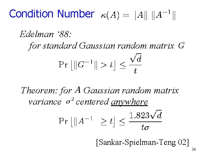
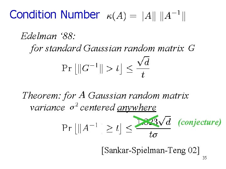
Condition Number Edelman ‘ 88: for standard Gaussian random matrix Theorem: for Gaussian random matrix variance centered anywhere [Sankar-Spielman-Teng 02] 34

Condition Number Edelman ‘ 88: for standard Gaussian random matrix Theorem: for Gaussian random matrix variance centered anywhere (conjecture) [Sankar-Spielman-Teng 02] 35

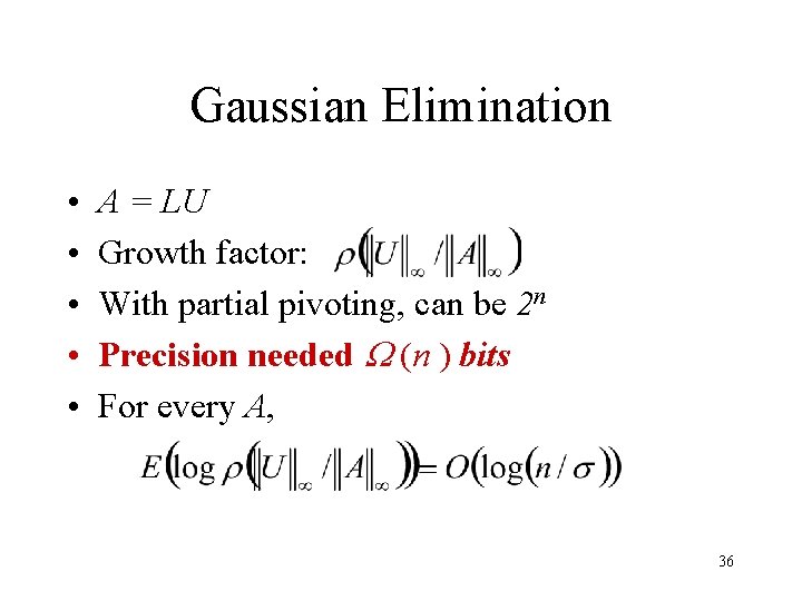
Gaussian Elimination • • • A = LU Growth factor: With partial pivoting, can be 2 n Precision needed (n ) bits For every A, 36

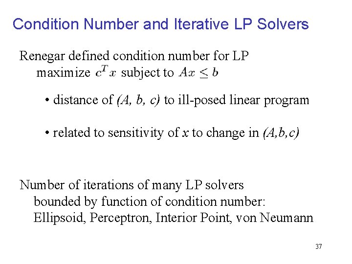
Condition Number and Iterative LP Solvers Renegar defined condition number for LP maximize subject to • distance of (A, b, c) to ill-posed linear program • related to sensitivity of x to change in (A, b, c) Number of iterations of many LP solvers bounded by function of condition number: Ellipsoid, Perceptron, Interior Point, von Neumann 37

Smoothed Analysis of Perceptron Algorithm [Blum-Dunagan 01] Theorem: For perceptron algorithm Bound through “wiggle room”, a condition number Note: slightly weaker than a bound on expectation 38

Smoothed Analysis of Renegar’s Cond Number Theorem: [Dunagan-Spielman-Teng 02] Corollary: smoothed complexity of interior point method is for accuracy e Compare: worst-case complexity of IPM is iterations, note 39

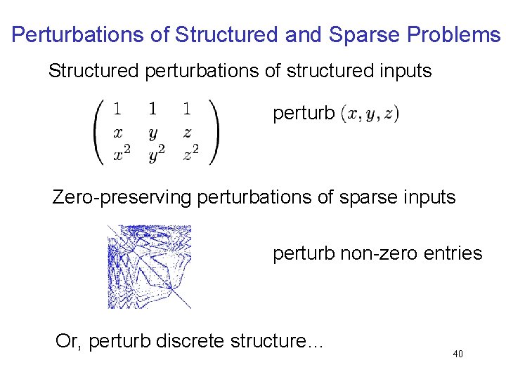
Perturbations of Structured and Sparse Problems Structured perturbations of structured inputs perturb Zero-preserving perturbations of sparse inputs perturb non-zero entries Or, perturb discrete structure… 40

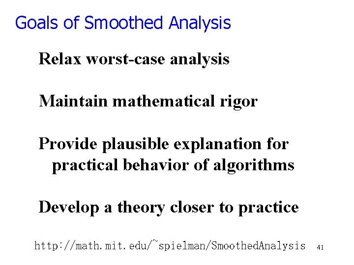
Goals of Smoothed Analysis Relax worst-case analysis Maintain mathematical rigor Provide plausible explanation for practical behavior of algorithms Develop a theory closer to practice http: //math. mit. edu/~spielman/Smoothed. Analysis 41

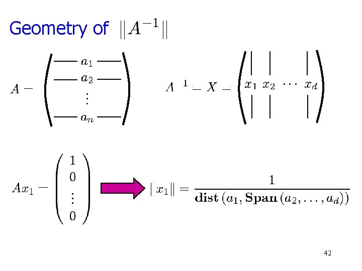
Geometry of 42

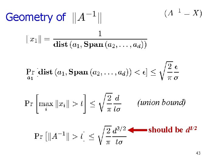
Geometry of (union bound) should be d 1/2 43

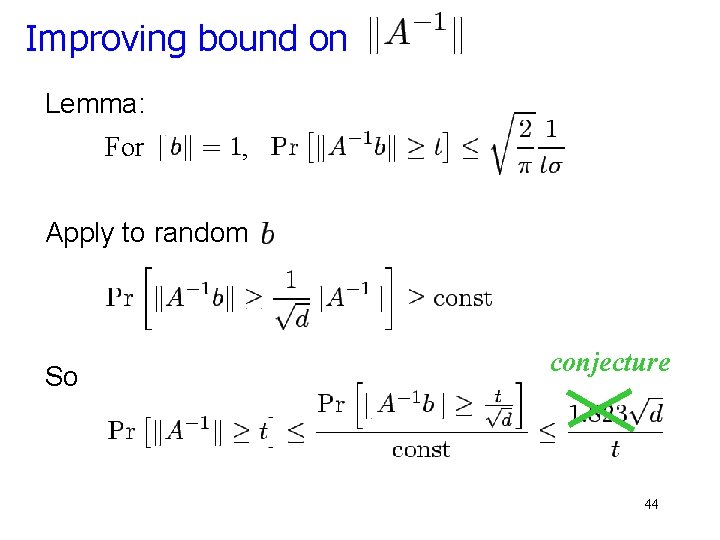
Improving bound on Lemma: For , Apply to random So conjecture 44

Smoothed Analysis of Renegar’s Cond Number Theorem: [Dunagan-Spielman-Teng 02] Corollary: smoothed complexity of interior point method is for accuracy e conjecture Compare: worst-case complexity of IPM is iterations, note 45