The Simplex Tableau Summary and Sensitivity Analysis Applied

The Simplex Tableau Summary and Sensitivity Analysis Applied Operations Research 2020 -2021 Susana Barreiro 26 March 2021

The Simplex Tableau Implementation Summary

The Simplex Tableau • Elegant algorithmic engine for solving linear programs • Allows examining the internal mechanics of the simplex method in a table representation of the basis at any cornerpoint • The tableau contains all the information that is needed to decide on the exchange of variables that drives the movement between cornerpoints as the simplex method goes forward • Tableau calculations are similar to the calculations carried out by computer implementations of the simplex method (e. g. SOLVER) • Allows understanding how the computer: - does its work on large LPs - calculations can go wrong

The Simplex Tableau - implementation • 1 Find an initial cornerpoint feasible solution (if none is found, then the model is infeasible, so exit) • 2 Iterate until the stopping conditions are met: • 2. 1 Are we optimal yet? Look at the current version of the objective function to see if an entering basic variable is available. If none is available, then exit with the current basic feasible solution as the optimum solution • 2. 2 Select entering basic variable: choose the nonbasic variable that gives the fastest rate of increase in the objective function value • 2. 3 Select the leaving basic variable by applying the minimum ratio test • 2. 4 Update the equations to reflect the new basic feasible solution • 2. 5 Go to Step 2. 1.

The Simplex Tableau - implementation • The most important thingd about Tableau: • exactly 1 basic variable per equation • the coefficient of the basic variable is always exactly +1, and the coefficients above and below the basic variable in the same column are all 0 • Z is treated as the basic variable for the objective function row (equation 0) A big advantage of the Tableau - you can always read the current solution directly from it (nonbasic variables are always zero)

The Simplex Tableau - implementation • Entering basic variable the one that gives the fastest rate of increase in the objective function value: Z = 15 x 1+ 10 x 2 -> the obvious entering basic variable is x 1 In the tableau, however, Z – 15 x 1 – 10 x 2 = 0 rule: choose the variable in the objective function row that has the most negative value Must check for negative coefficients in the objective function row, if so we are not optimal yet: the simplex iterations must continue The column for the entering basic variable is called the pivot column

The Simplex Tableau - implementation • Leaving basic variable • Is associated with the row that has the lowest ratio test - the pivot row. The minimum ratio test (mrt) determines which constraint most limits the increase in the value of the entering basic variable. • For the mrt look only at the entries in the pivot column (RHS/coeff pivot column) • Two special cases regarding the coefficient of the entering basic variable: is zero: mrt = “no limit” is negative: mrt = “no limit” choosing the leaving basic variable via the minimum ratio test is the same as finding out which constraint you first bump into as the entering basic variable increases in value Why is the mrt never applied to the objective function row? It is not a constraint, so it can never limit the increase in the value of the entering basic variable. It goes along for the ride, just for quantifying the objective along the way

The Simplex Tableau - implementation • Updating the table: • Replace the leaving basic variable listed for the pivot row by the entering basic variable. • Force the entering variable vector to take the shape of the leaving variable vector • The tableau element where the pivot row and the pivot column intersect is known as the pivot element. • Eliminate all of the coefficients in the pivot column except the pivot element that must take the value 1. This is done by simple Gaussian operations

The Simplex Tableau - implementation Tie for the entering basic variable • This means that both variables will increase Z at the same rate. • How to handle this situation? choose the entering basic variable arbitrarily, because there is no good way to determine in advance which selection will reach the optimum solution in the smallest number of pivots Tie for the leaving basic variable • Means there are two constraints (with their corresponding basic variables) that are tied as the first constraints you bump into • Technically speaking, the basic feasible solutions will be different, because each will define a different partitioning of the variables into basic and nonbasic sets. • Again, simply choose arbitrarily. • Both variables must be zero simultaneously because both constraints are active at that point • The basic feasible solution defines what is known as a degenerate solution. Degenerate solutions can lead to an infinite loop of solutions that traps the simplex solution method; this is known as cycling

The Simplex Tableau - implementation Suppose that all of the minimum ratio tests are tied at “no limit” • What does this mean? That no constraint puts a limit on the increase in the value of the entering basic variable! And consequently to the value of the objective function. • Your result might then show that you can make an infinite amount of profit but it usually means that you forgot a constraint. Problems of this type are called unbounded At the Optimum, the Coefficients of Some Nonbasic Variables are Zero in the Objective Function Row it means that choosing this variable as the entering basic variable increases Z at the rate of zero, i. e. it has no effect on Z! You have the same value of Z, but you will pivot to a different basic feasible solution. Two different basic feasible solutions with the same value of Z means that there must be multiple optimum solutions (at both of the two basic feasible solutions – cornerpoints- and at any point between those two solutions) To see the other optima, choose one of the nonbasic variables whose objective function coefficient is zero as the entering basic variable, and pivot to another basic feasible solution as you normally would

The Simplex Tableau - implementation Artificial variables • Have no physical meaning in the original problem and are introduced to allow obtaining a basic feasible solution for applying the simplex method. • To prevent them from becoming part of an optimal solution to the original problem, a very large “penalty” is introduced into the objective function by choosing a positive constant M as the artificial variable coefficient and forcing it to be 0 in the optimal solution. The same constant M is used for all artificial variables. • To achieve this, assign a -M penalty for maximization and +M penalty for minimization in the objective function. Maximize P = 2 x 1+ x 2 subject to: x 1 + x 2 ≤ 10 9 x 1 + x 2 ≥ 2 x 1 , x 2 ≥ 0 Maximize P = 2 x 1+ x 2 –Ma 1 subject to: x 1 + x 2 + s 1 = 10 9 x 1 + x 2 – s 2 + a 1 = 2 x 1, x 2, s 1, s 2, a 1 ≥ 0 Maximize P - 2 x 1 - x 2 +Ma 1 subject to: x 1 + x 2 + s 1 = 10 9 x 1 + x 2 – s 2 + a 1 = 2 x 1, x 2, s 1, s 2, a 1 ≥ 0

The Simplex Tableau - implementation • Relate the optimal solution of the modified problem to the original problem. A. if the modified problem has no optimal solution, the original problem has no optimal solution. B. if all artificial variables are 0 in the optimal solution to the modified problem, delete the artificial variables to find an optimal solution to the original problem C. if any artificial variables are nonzero in the optimal solution, the original problem has no optimal solution.

The Simplex Tableau An example

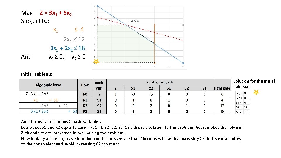
Max Z = 3 x 1 + 5 x 2 Subject to: x 1 ≤ 4 And 2 x 2 ≤ 12 3 x 1 + 2 x 2 ≤ 18 x 1 ≥ 0; x 2 ≥ 0 Initial Tableaux Solution for the initial Tableaux And 3 constraints means 3 basic variables. Lets us set x 1 and x 2 equal to zero => S 1=4, S 2=12, S 3=18 : this is a solution to the problem, but it makes the value of Z =0 and we are interested in maximizing the problem. Now looking at the objective function coefficients we see that Z increases faster by increasing X 2, but we must obey to the constraints and avoid increasing X 2 too much

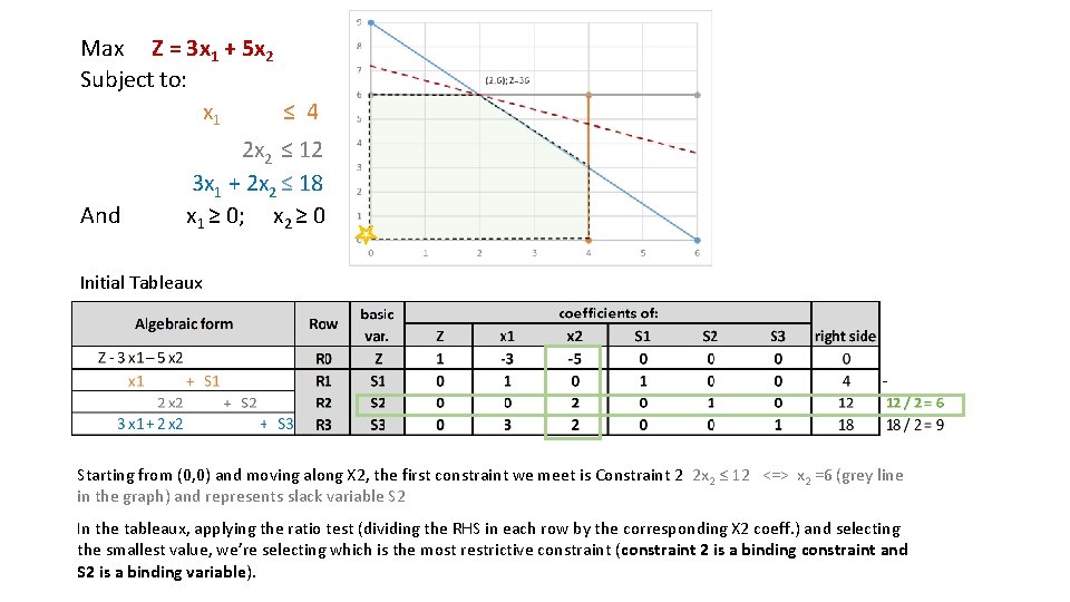
Max Z = 3 x 1 + 5 x 2 Subject to: x 1 ≤ 4 And 2 x 2 ≤ 12 3 x 1 + 2 x 2 ≤ 18 x 1 ≥ 0; x 2 ≥ 0 Initial Tableaux Starting from (0, 0) and moving along X 2, the first constraint we meet is Constraint 2 2 x 2 ≤ 12 <=> x 2 =6 (grey line in the graph) and represents slack variable S 2 In the tableaux, applying the ratio test (dividing the RHS in each row by the corresponding X 2 coeff. ) and selecting the smallest value, we’re selecting which is the most restrictive constraint (constraint 2 is a binding constraint and S 2 is a binding variable).

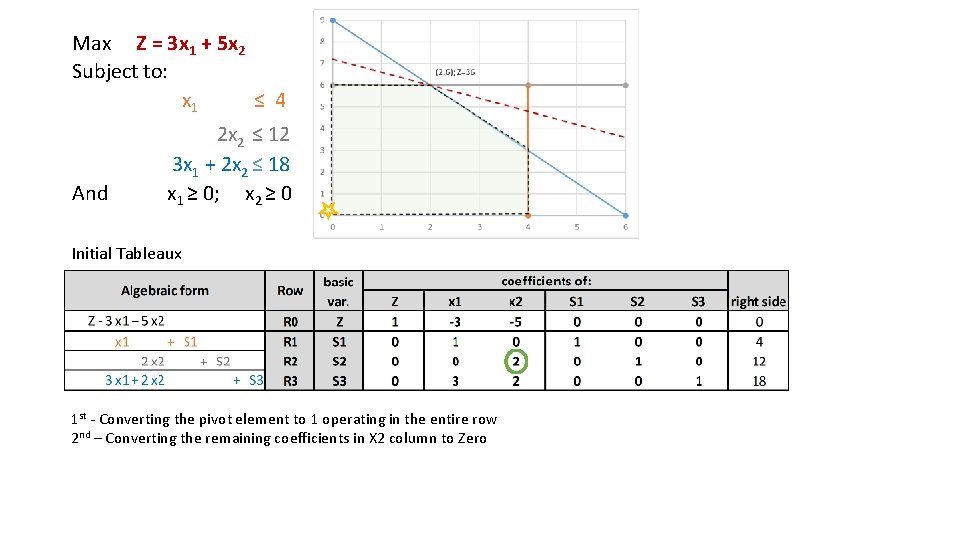
Max Z = 3 x 1 + 5 x 2 Subject to: x 1 ≤ 4 And 2 x 2 ≤ 12 3 x 1 + 2 x 2 ≤ 18 x 1 ≥ 0; x 2 ≥ 0 Initial Tableaux 1 st - Converting the pivot element to 1 operating in the entire row 2 nd – Converting the remaining coefficients in X 2 column to Zero

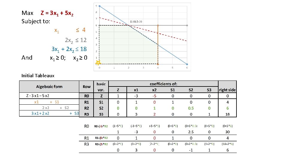
Max Z = 3 x 1 + 5 x 2 Subject to: x 1 ≤ 4 And 2 x 2 ≤ 12 3 x 1 + 2 x 2 ≤ 18 x 1 ≥ 0; x 2 ≥ 0 Initial Tableaux

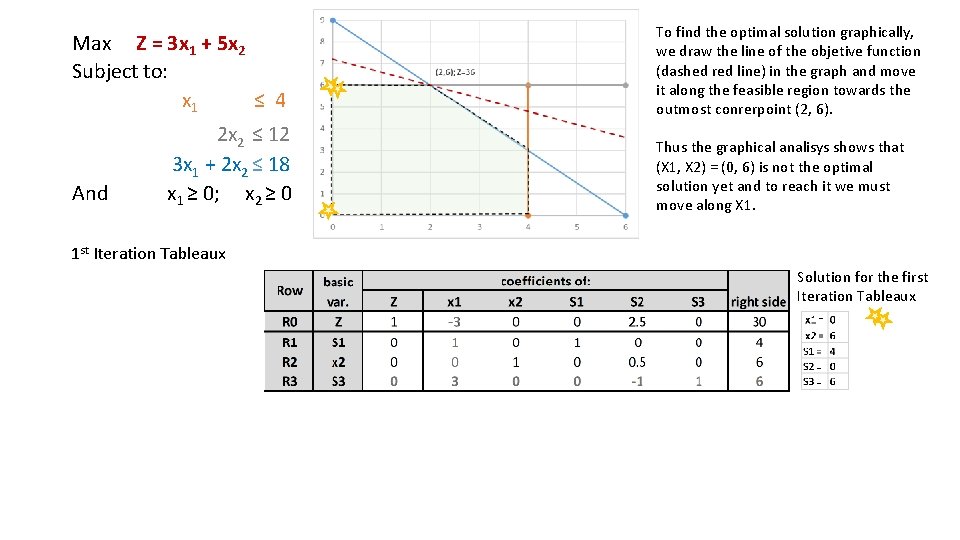
Max Z = 3 x 1 + 5 x 2 Subject to: x 1 ≤ 4 And 2 x 2 ≤ 12 3 x 1 + 2 x 2 ≤ 18 x 1 ≥ 0; x 2 ≥ 0 To find the optimal solution graphically, we draw the line of the objetive function (dashed red line) in the graph and move it along the feasible region towards the outmost conrerpoint (2, 6). Thus the graphical analisys shows that (X 1, X 2) = (0, 6) is not the optimal solution yet and to reach it we must move along X 1. 1 st Iteration Tableaux Solution for the first Iteration Tableaux

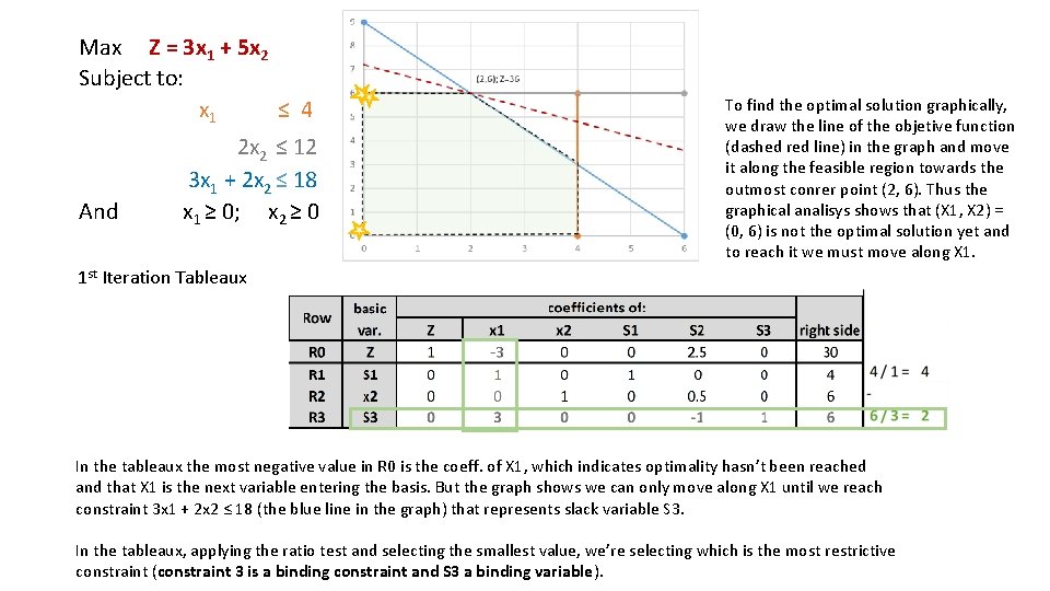
Max Z = 3 x 1 + 5 x 2 Subject to: x 1 ≤ 4 And 2 x 2 ≤ 12 3 x 1 + 2 x 2 ≤ 18 x 1 ≥ 0; x 2 ≥ 0 To find the optimal solution graphically, we draw the line of the objetive function (dashed red line) in the graph and move it along the feasible region towards the outmost conrer point (2, 6). Thus the graphical analisys shows that (X 1, X 2) = (0, 6) is not the optimal solution yet and to reach it we must move along X 1. 1 st Iteration Tableaux In the tableaux the most negative value in R 0 is the coeff. of X 1, which indicates optimality hasn’t been reached and that X 1 is the next variable entering the basis. But the graph shows we can only move along X 1 until we reach constraint 3 x 1 + 2 x 2 ≤ 18 (the blue line in the graph) that represents slack variable S 3. In the tableaux, applying the ratio test and selecting the smallest value, we’re selecting which is the most restrictive constraint (constraint 3 is a binding constraint and S 3 a binding variable).

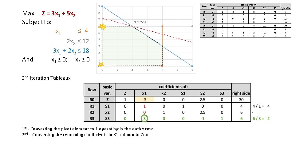
Max Z = 3 x 1 + 5 x 2 Subject to: x 1 ≤ 4 And 2 x 2 ≤ 12 3 x 1 + 2 x 2 ≤ 18 x 1 ≥ 0; x 2 ≥ 0 2 nd Iteration Tableaux 1 st - Converting the pivot element to 1 operating in the entire row 2 nd – Converting the remaining coefficients in X 1 column to Zero

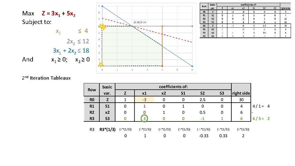
Max Z = 3 x 1 + 5 x 2 Subject to: x 1 ≤ 4 And 2 x 2 ≤ 12 3 x 1 + 2 x 2 ≤ 18 x 1 ≥ 0; x 2 ≥ 0 2 nd Iteration Tableaux

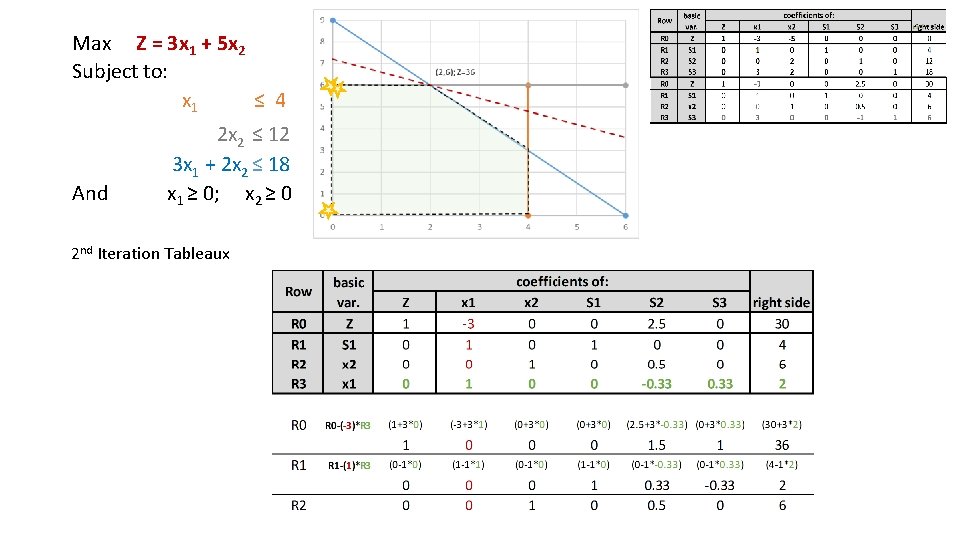
Max Z = 3 x 1 + 5 x 2 Subject to: x 1 ≤ 4 And 2 x 2 ≤ 12 3 x 1 + 2 x 2 ≤ 18 x 1 ≥ 0; x 2 ≥ 0 2 nd Iteration Tableaux

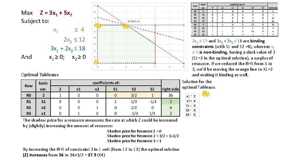
Max Z = 3 x 1 + 5 x 2 Subject to: x 1 ≤ 4 And 2 x 2 ≤ 12 3 x 1 + 2 x 2 ≤ 18 x 1 ≥ 0; x 2 ≥ 0 2 x 2 ≤ 12 and 3 x 1 + 2 x 2 ≤ 18 are binding constraints (with S 1 and S 2 =0), whereas x 1 ≤ 4 is non-binding, having a slack value of 2 (S 1=2 in the optimal solution), a surplus of resource. If we reduced the RHS from 4 to 2, we’d be moving the orange line to X 1=2 and making it binding as well. Solution for the optimal Tableaux Optimal Tableaux The shadow price for a resource measures the rate at which Z could be increased by (slightly) increasing the amount of resource: Shadow price for Resource 1 = 0 Shadow price for Resource 2 = 3/2 = 1+1/2 Shadow price for Resource 3 = 1 By increasing the RHS of constraint 2 in 1 unit (from 12 to 13) the optimal solution (Z) increases from 36 to 36+3/2 = 37. 5 (K€)

The Simplex Tableau Sensitivity Analysis

Sensitivity Analysis – Simplex tableau • We wish to analyze the effect of changing various elements of the problem data without re-solving the LPP on the optimal solution using only the initial and final tableaus • The type of results that can be derived in this way are conservative, in the sense that they provide sensitivity analysis for small enough changes in the problem so that the same decision variables remain basic, but not for larger changes in the data

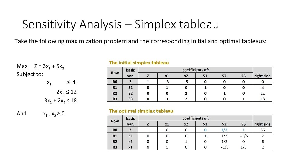
Sensitivity Analysis – Simplex tableau Take the following maximization problem and the corresponding initial and optimal tableaus: Max Z = 3 x 1 + 5 x 2 Subject to: x 1 ≤ 4 The initial simplex tableau 2 x 2 ≤ 12 3 x 1 + 2 x 2 ≤ 18 And x 1 , x 2 ≥ 0 The optimal simplex tableau

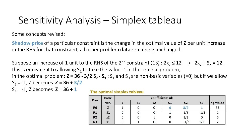
Sensitivity Analysis – Simplex tableau Some concepts revised: Shadow price of a particular constraint is the change in the optimal value of Z per unit increase in the RHS for that constraint, all other problem data remaining unchanged. Suppose an increase of 1 unit to the RHS of the 2 nd constraint (13) : 2 x 2 ≤ 12 -> 2 x 2 + S 2 = 12, this is equivalent to allowing S 2 to take the value -1 in the original problem, in the optimal problem: Z = 36 - 3/2 S 2 - S 3 ; S 2 and S 3 are non-basic variables (=0) but if we allow S 2 = -1, Z becomes Z = 36 + 3/2 S 3 = -1, Z becomes Z = 36 + 1 The optimal simplex tableau

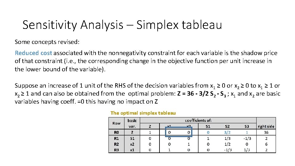
Sensitivity Analysis – Simplex tableau Some concepts revised: Reduced cost associated with the nonnegativity constraint for each variable is the shadow price of that constraint (i. e. , the corresponding change in the objective function per unit increase in the lower bound of the variable). Suppose an increase of 1 unit of the RHS of the decision variables from x 1 ≥ 0 or x 2 ≥ 0 to x 1 ≥ 1 or x 2 ≥ 1 and can also be obtained from the optimal problem: Z = 36 - 3/2 S 2 - S 3 ; x 1 and x 2 are basic variables having coeff. =0 this having no impact on Z The optimal simplex tableau

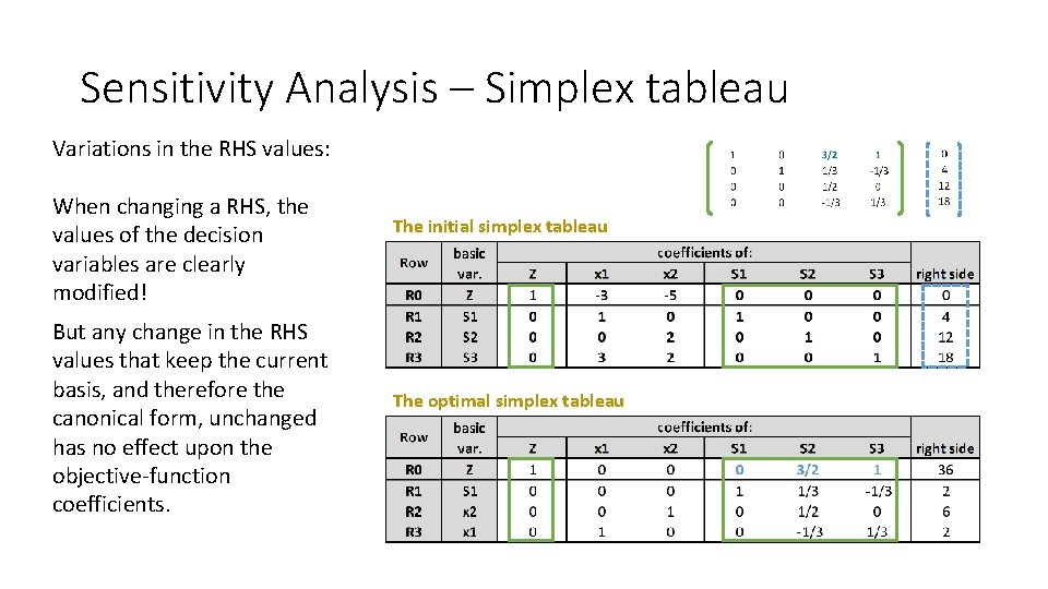
Sensitivity Analysis – Simplex tableau Variations in the RHS values: When changing a RHS, the values of the decision variables are clearly modified! But any change in the RHS values that keep the current basis, and therefore the canonical form, unchanged has no effect upon the objective-function coefficients. The initial simplex tableau The optimal simplex tableau

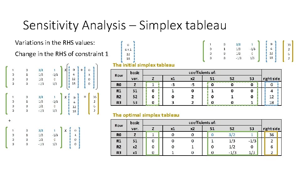
Sensitivity Analysis – Simplex tableau Variations in the RHS values: Change in the RHS of constraint 1 x x The initial simplex tableau + = The optimal simplex tableau + x

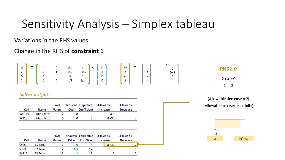
Sensitivity Analysis – Simplex tableau Variations in the RHS values: Change in the RHS of constraint 1 + x = + 0 λ 0 0 = 0 2+ λ 0 0 RHS ≥ 0 2+λ=0 λ = -2 Solver output: (Allowable decrease = 2) (Allowable increase = infinity)

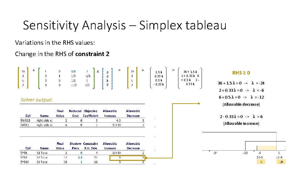
Sensitivity Analysis – Simplex tableau Variations in the RHS values: Change in the RHS of constraint 2 + x 0 0 λ 0 = + 1. 5 λ 0. 33 λ 0. 5 λ - 0. 33 λ = 36 + 1. 5 λ 2 + 0. 33 λ 6 + 0. 5 λ 2 0. 33 λ RHS ≥ 0 36 + 1. 5 λ = 0 -> λ = -24 2 + 0. 33 λ = 0 -> λ = -6 Solver output: 6 + 0. 5 λ = 0 -> λ = -12 (Allowable decrease) 2 - 0. 33 λ = 0 -> λ = 6 (Allowable increase)

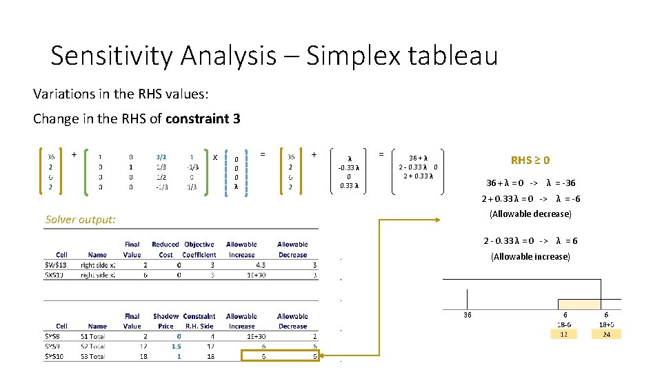
Sensitivity Analysis – Simplex tableau Variations in the RHS values: Change in the RHS of constraint 3 + x 0 0 0 λ = + λ -0. 33 λ 0 0. 33 λ = 36 + λ 2 - 0. 33 λ 0 2 + 0. 33 λ RHS ≥ 0 36 + λ = 0 -> λ = -36 2 + 0. 33 λ = 0 -> λ = -6 Solver output: (Allowable decrease) 2 - 0. 33 λ = 0 -> λ = 6 (Allowable increase)

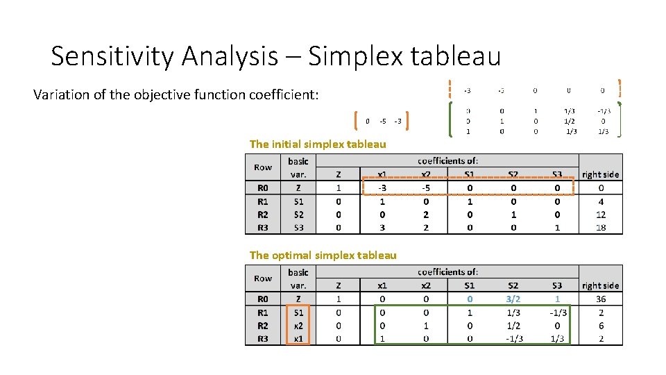
Sensitivity Analysis – Simplex tableau Variation of the objective function coefficient: 0 -5 -3 The initial simplex tableau The optimal simplex tableau

Sensitivity Analysis – Simplex tableau Variation of the objective function coefficient: Change in coeff. of x 1 (c 1) The initial simplex tableau x = The optimal simplex tableau

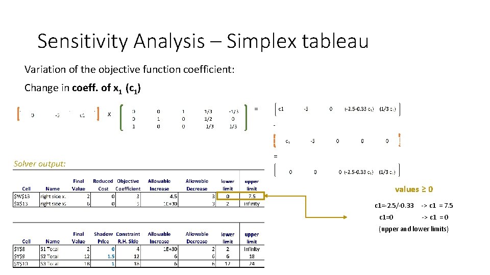
Sensitivity Analysis – Simplex tableau Variation of the objective function coefficient: Change in coeff. of x 1 (c 1) x = - Solver output: = values ≥ 0 c 1=-2. 5/-0. 33 c 1=0 -> c 1 = 7. 5 -> c 1 = 0 (upper and lower limits)

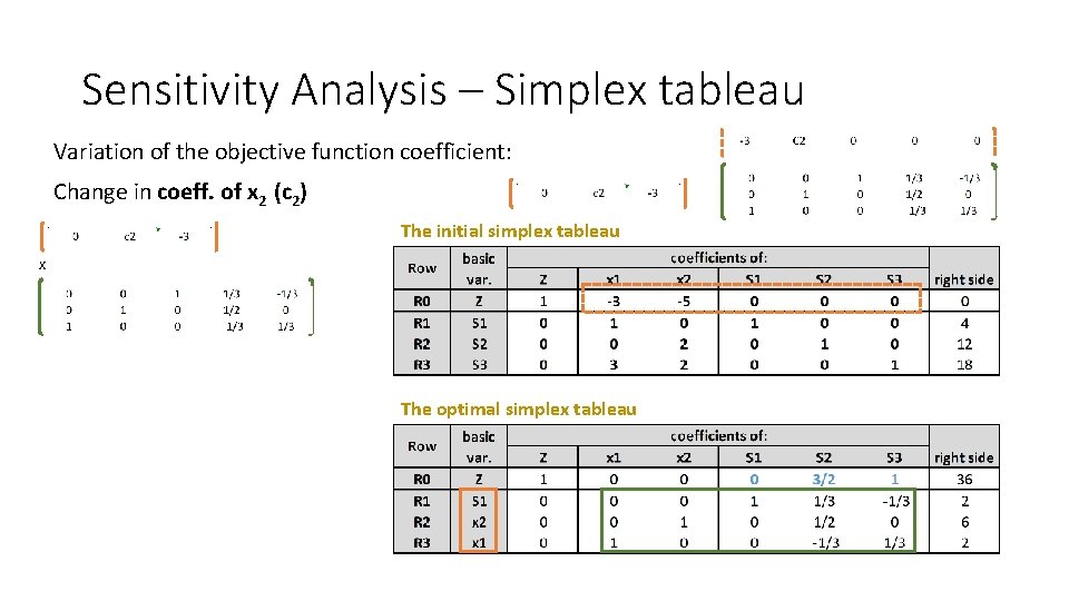
Sensitivity Analysis – Simplex tableau Variation of the objective function coefficient: Change in coeff. of x 2 (c 2) The initial simplex tableau x The optimal simplex tableau

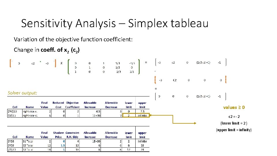
Sensitivity Analysis – Simplex tableau Variation of the objective function coefficient: Change in coeff. of x 2 (c 2) x = - Solver output: = values ≥ 0 c 2 = -2 (lower limit = 2 ) (upper limit = infinity)