THE SIMPLEX METHOD Chapter Four History of Linear

THE SIMPLEX METHOD Chapter Four

History of Linear Programming George Dantzig 1914 - 2008 George B. Dantzig developed such a method in 1947 while being assigned to the U. S. military. Ideally suited to computer use, the method is used routinely on applied problems involving hundreds and even thousands of variables and problem constraints.

STANDARD LINEAR PROGRAMMING FORM General Simplex LP model: Minimize : Subject to : F(X) = ci xi aji xi = bj j = 1, m xi 0 i = 1, n In order to get and maintain this form, use • slack, if Ax b, then A. x + slack = b • surplus, if Ax b, then A. x - surplus = b • artificial variables (to generate the canonical form) IMPORTANT: Simplex only deals with equalities

Nonnegative design variables • Replacing variable Xi by two positive variables and taking their difference Xi = X’i – X”i X’i ≥ 0 X”i ≥ 0 i = 1, n (Doubled number of design variables ) • An alternative approach would be to add a constant to each of the design variables Xi X i = X ’i – Q i (If an unreasonably large value of Qi is used , considerable numerical ill-conditioning appear )

Convert to Standard Form a 11 x 1 + a 12 x 2 + • • • + a 1 n xn ≤ b 1, a 11 x 1 + a 12 x 2 + • • • + a 1 n xn + xn+1 = b 1, a 21 x 1 + a 22 x 2 + • • • + a 2 n xn ≥ b 2, a 21 x 1 + a 22 x 2 + • • • + a 2 n xn - xn+2 = b 2, am 1 x 1 + am 2 x 2 + • • • + amn xn ≤ bm, am 1 x 1 + am 2 x 2 + • • • + amn xn + xn+m = bm, • Matrix form of linear programming problem Minimize : f = c. X Subject to : AX=b Xi ≥ 0 i= 1, n

Graphing 2 -Dimensional LPs Optimal Solution y Example 1: 4 Maximize x+y Subject to: x + 2 y 2 x 3 y 4 x 0 y 0 3 Feasible Region 2 1 0 x 0 1 2 3

Graphing 2 -Dimensional LPs y Example 2: 4 Minimize ** Multiple Optimal Solutions! x-y Subject to: 1/3 x + y 4 -2 x + 2 y 4 3 2 Feasible Region x 3 x 0 y 0 1 0 0 1 2 3 x

Graphing 2 -Dimensional LPs y Example 3: 40 Minimize x + 1/3 y Subject to: x + y 20 -2 x + 5 y 150 x 5 x 0 y 0 Optimal Solution 30 Feasible Region 20 10 x 0 0 10 20 30 40

Do We Notice Anything From These 3 Examples? y y y 4 4 40 3 3 30 2 2 20 1 1 10 0 0 1 2 3 x 0 0 10 20 x 30 If an optimal solution exists, there is always a corner point optimal solution! 40

Graphing 2 -Dimensional LPs Second Example 1: Corner pt. Maximize x+y Subject to: x + 2 y 2 x 3 Optimal Solution y 4 3 Feasible Region y 4 x 0 y 0 2 1 Initial Corner pt. 0 x 0 1 2 3 And We Can Extend this to Higher Dimensions

POSSIBLE SOLUTION TO THE LINEAR PROGRAMMING PROBLEM

POSSIBLE SOLUTION TO THE LINEAR PROGRAMMING PROBLEM

POSSIBLE SOLUTION TO THE LINEAR PROGRAMMING PROBLEM

POSSIBLE SOLUTION TO THE LINEAR PROGRAMMING PROBLEM

THE SIMPLEX METHOD X 1 X 2 X 3 … Xn Xn+1 … X n+k a 1, 1 a 1, 2 a 1, 3 … a 1, n 1 … a 2, 1 a 2, 2 a 2, 3 … a 2, n . . . ar, 1 ar, 2 Xn+m = b 0 0 = b 1 … 1 0 = b 2 . . . ar, 3 … ar, n 0 … 0 = br am, 1 am, 2 am, 3 … am, n 0 … 1 = bm … cn 0 … 0 = f-f 0 c 1 c 2 c 3 … This is the objective Function row

1. Canonical Form Matrix with one element in each row and column equal to unit It’s dimension is m by m ( No. of constraints) Each table must start with a canonical form 2. Basic Variables which are within canonical form 3. Basis Set of basic variables 4. Non Basic Variables which are out of canonical form 5. f 0 The constant term in objective function 6. Data of each table Each basic variable is equal to it’s bi Non basic variables are zeroes Objective function is equal to f 0 Ci for slack variables are the Lagrange coefficient of related constraints

minimize F =-4 x 1 - x 2 + 50 subject to : The pivotal row x 1 - x 2 ≤ 2 x 1 + 2 x 2 ≤ 8 x 1, x 2, x 3, x 4 x 1 x 2 x 3 x 4 = b 1 -1 1 0 = 2 1 2 0 1 = 8 -4 -1 0 0 = F-50 0 This is the most negative coefficient it’s column is called the pivotal column.

x 1 x 2 x 3 x 4 = b 1 -1 1 0 = 2 0 3 -1 1 = 6 0 -5 4 0 = F-42 x 1 x 2 x 3 x 4 = b 1 0 2/3 1/3 = 4 0 1 -1/3 = 2 0 0 7/3 5/3 = F-32

minimize F =-x 1 + x 2 + 30 subject to : x 1 - x 2 ≤ 2 x 1 + 2 x 2 ≤ 8 x 1, x 2, x 1 x 2 x 3 x 4 = b 1 -1 1 0 = 2 1 2 0 1 = 8 -1 1 0 0 = F-30 x 3, x 4 0

x 1 x 2 x 3 x 4 = b 1 -1 1 0 = 2 0 3 -1 1 = 6 0 0 1 0 = F-28

minimize F =-4 x 1 - x 2 + 50 subject to : x 1 - x 2 ≤ 2 x 1, x 2, x 3 x 1 x 2 x 3 = b 1 -1 1 = 2 -4 -1 0 = F-50 0

x 1 x 2 x 3 = b 1 -1 1 = 2 0 -5 4 = F-42

Example 1 minimize subject to : F = -4 x 1 - x 2 + 50 x 1 - x 2 ≤ -5 x 1 + 2 x 2 ≤ 8 x 1, x 2 0

minimize subject to : F = -4 x 1 - x 2 + 50 x 1 - x 2 ≤ -5 x 1 + 2 x 2 ≤ 8 x 1, x 2 0 1) -x 1 + x 2 ≥ 5 x 1 + 2 x 2 ≤ 8 -x 1 + x 2 – x 3+ x 5= 5 x 1 + 2 x 2 + x 4 =8 2) x 1 - x 2 ≤ -5 x 1 + 2 x 2 ≤ 8 x 1 - x 2 + x 3= -5 x 1 + 2 x 2 + x 4= 8 -x 1 + x 2 – x 3+ x 5=5

x 1 x 2 x 3 x 4 x 5 = b -1 1 -1 0 1 = 5 1 2 0 1 0 = 8 -4 -1 0 0 0 = F-50 0 0 1 = w

x 1 x 2 x 3 x 4 x 5 = b -1 1 -1 0 1 = 5 1 2 0 1 0 = 8 -4 -1 0 0 0 = F-50 1 -1 1 0 0 = W-5

x 1 x 2 x 3 -3/2 0 1/2 x 5 = b -1 -1/2 1 = 1 1 0 1/2 0 = 4 -7/2 0 0 1/2 0 = F-46 3/2 0 1 1/2 0 = W-1 No solution x 4

Example 2 minimize F = -4 x 1 - x 2 + 50 subject to : x 1 - x 2 = 2 x 1 + 2 x 2 ≤ 8 x 1, x 2, x 3, x 4 0 minimize F = -4 x 1 - x 2 + 50 subject to : x 1 - x 2 + x 3 = 2 x 1 + 2 x 2 + x 4 = 8 x 1, x 2, x 3, x 4 0

Artificial Variable Phase : I x 1 x 2 x 3 x 4 = b 1 -1 1 0 = 2 1 2 0 1 = 8 -4 -1 0 0 = F-50 0 0 1 0 = W

x 1 x 2 x 3 x 4 = b 1 -1 1 0 = 2 1 2 0 1 = 8 -4 -1 0 0 = F-50 -1 1 0 0 = W-2 x 1 x 2 x 3 x 4 = b 1 -1 1 0 = 2 0 3 -1 1 = 6 0 -5 4 0 = F-42 0 0 1 0 = W

Phase : II x 1 x 2 x 3 x 4 = b 1 -1 1 0 = 2 0 3 -1 1 = 6 0 -5 4 0 = F-42 0 0 1 0 = W x 1 x 2 x 4 = b 1 -1 0 = 2 0 3 1 = 6 0 -5 0 = F-42

x 1 x 2 x 4 = b 1 0 1/3 = 4 0 1 1/3 = 2 0 0 5/3 = F-32

Example 2 minimize F = -4 x 1 - x 2 + 50 subject to : x 1 - x 2 = 2 x 1 + 2 x 2 ≤ 8 x 1, x 2 0 x 1 - x 2 = 2 x 1 - x 2 ≤ 2 x 1 - x 2 + x 3 = 2 x 1 - x 2 – x 4 + x 5 =2 x 1 + 2 x 2 + x 6 = 8 x 1, x 2, x 3, x 4 , x 5, x 6 0

Artificial Variable Phase : I x 1 x 2 x 3 x 4 x 5 x 6 = b 1 -1 1 0 0 0 = 2 1 -1 0 -1 1 0 = 2 1 2 0 0 0 1 = 8 -4 -1 0 0 = F-50 0 0 1 0 = W

Artificial Variable Phase : I x 1 x 2 x 3 x 4 x 5 x 6 = b 1 -1 1 0 0 0 = 2 1 -1 0 -1 1 0 = 2 1 2 0 0 0 1 = 8 -4 -1 0 0 = F-50 -1 1 0 0 = W-2

Artificial Variable Phase : I x 1 x 2 x 3 x 4 x 5 x 6 = b 0 0 1 1 -1 0 = 0 1 -1 0 -1 1 0 = 2 0 3 0 1 -1 1 = 6 0 -5 0 -4 4 0 = F-42 0 0 1 0 = W

Phase : 2 x 1 x 2 x 3 x 4 x 6 = b 0 0 1 1 0 = 0 1 -1 0 = 2 0 3 0 1 1 = 6 0 -5 0 -4 0 = F-42

Phase : 2 x 1 x 2 x 3 x 4 x 6 = b 0 0 1 1 0 = 0 1 0 0 -2/3 1/3 = 4 0 1/3 1/3 = 2 0 0 0 -7/3 5/3 = F-32

Phase : 2 X 1 =4 X 2 =2 X 4 =0 X 6 =0 x 1 x 2 x 3 x 4 x 6 = b 0 0 1 1 0 = 0 1 0 2/3 0 1/3 = 4 0 1 -1/3 0 1/3 = 2 0 0 7/3 0 5/3 = F-32 F =32 λ 1 =7/3 λ 2 =5/3

The simplex Algorithm • Phase II ( problem is in canonical form ) 1. Find the minimum ci , i=1, n. Let the subscript k denote this variable with cost coefficient ck. If ck is nonnegative, go to step 5. ck is negative. now find the minimum bj/ajk, j=1, m for all positive ajk. if all ajk nonpositive , the solution is unbounded. therefore , go to step 5. otherwise, let the subscript r denote the row corresponding this minimum. ark is now the pivot element. Pivot on ark , first divide row r by ark. next subtract ajk times row r from row j , j=1, m+1 and j≠r. Go to step 1 and repeat. The solution is complete. 2. 3. 4. 5.

• If all ci associated with nonbasic variables are positive , the solution is unique. • If some ci associated with nonbasic variables is zero , the solution is not unique. • If some ci is negative , the solution is unbounded.

The simplex Algorithm Phase I ( produce of canonical form ) 1. Add artificial variables as necessary to achieve canonical form. 2. Create a new objective function w equal to the sum of the artificial variables. 3. Minimize w using the same as phase II

Duality Every linear programming problem is convex and separable so it can be solve in Primal or Dual form Simplex method search each corner of feasible area so less corner is desirable Less constraints, less corners Problem with number of constraints less than number of design variables is desirable

• Primal Problem P Minimize F = C. X + F 0 subject to Ax ≤ b xi 0 i =1, n • Dual Problem D Maximize L(λ) = -b. T. λ + F 0 subject to AT. λ ≥ -C T λj≥ 0 j=1, m optimum value is F* optimum value is L* Theorem. (Strong Duality) If both P and D are feasible, then F* = L*.

PRIMAL PROBLEM: Minimize subject to : F (X) = -4 x 1 - x 2 + 50 x 1 - x 2 ≤ 2 x 1 + 2 x 2 ≤ 8 x 1 + x 2 ≤ 10 -5 x 1 + x 2 ≤ 5 x 1 0 , x 2 0 DUAL PROBLEM: Maximize L(λ) = -2λ 1 -8 λ 2 -10 λ 3 -5 λ 4 + 50 Subject to : λ 1 + λ 2 + λ 3 -5λ 4 4 -λ 1 + 2 λ 2 + λ 3 + λ 4 1 λ i 0 i=1, 4

Primal and dual relationship

Example minimize F = -4 x 1 - x 2 + 50 subject to : x 1 - x 2 = 2 x 1 + 2 x 2 ≤ 8 x 1, x 2, x 3, x 4 0 Artificial Variable Phase : I x 1 x 2 x 3 x 4 = b 1 -1 1 0 = 2 1 2 0 1 = 8 -4 -1 0 0 = F-50 0 0 1 0 = W

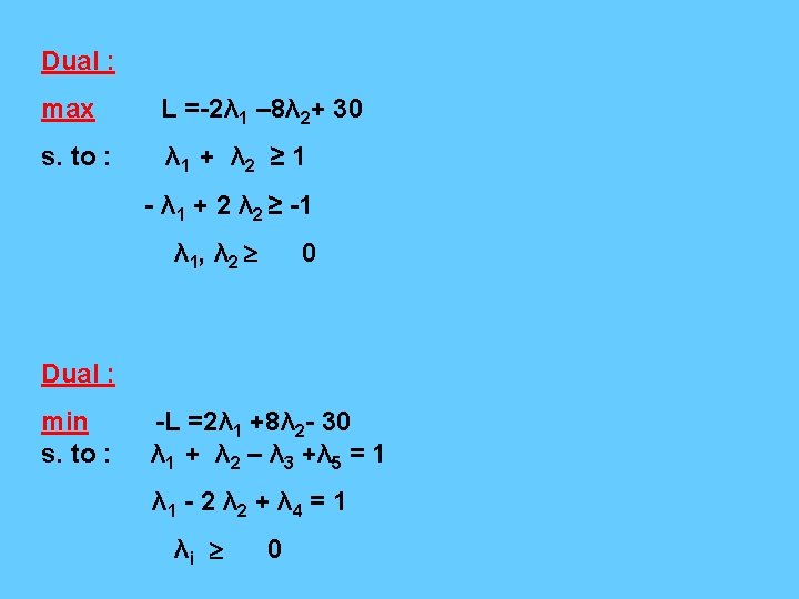
minimize F = -4 x 1 - x 2 + 50 subject to : x 1 - x 2 = 2 x 1 + 2 x 2 ≤ 8 x 1, x 2 0 Primal mode :

Dual mode : Unrestricted in sign

Dual mode :

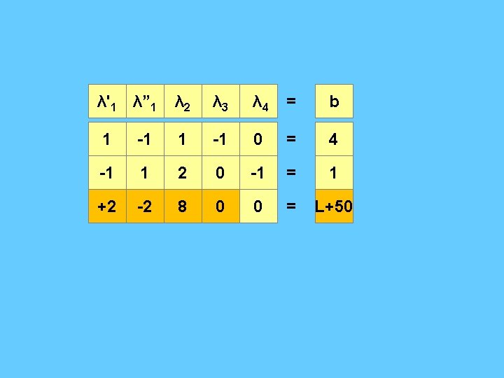
Artificial Variables λ'1 λ” 1 λ 2 λ 3 λ 4 λ 5 λ 6 = b 1 -1 0 1 0 = 4 -1 1 2 0 -1 0 1 = 1 2 -2 8 0 0 = L+50 0 0 1 1 = W

Artificial Variables λ'1 λ” 1 λ 2 λ 3 λ 4 λ 5 λ 6 = b 1 -1 0 1 0 = 4 -1 1 2 0 -1 0 1 = 1 2 -2 8 0 0 = L+50 0 0 -3 1 1 0 0 = W-5

λ'1 λ” 1 λ 2 λ 3 λ 4 λ 5 λ 6 = b 3/2 -3/2 0 -1 1/2 1 -1/2 = 7/2 -1/2 1 0 -1/2 0 1/2 = 1/2 -6 0 0 4 0 -4 = L+46 -3/2 0 1 -1/2 0 3/2 = W-7/2 6

λ'1 λ” 1 λ 2 λ 3 λ 4 λ 5 λ 6 = b 1 -1 0 -2/3 1/3 2/3 -1/3 = 7/3 0 0 1 -1/3 1/3 = 5/3 0 0 0 4 2 -4 -2 = L+32 0 0 0 1 1 = End of phase 1 W

λ'1 λ” 1 λ 2 λ 3 λ 4 = b 1 -1 0 -2/3 1/3 = 7/3 0 0 1 -1/3 = 5/3 0 0 0 4 2 λ 1=λ'1 - λ” 1=7/3 – 0 = 7/3 λ 2=5/3 λ 3= 0 λ 4= 0 x 1= 4 x 2= 2 Min : L = -32 Max : -L = 32 = L+32 End of phase 2

minimize F = -4 x 1 - x 2 + 50 subject to : x 1 - x 2 = 2 x 1 + 2 x 2 ≤ 8 x 1, x 2 0 Primal mode : minimize F = -4 x 1 - x 2 + 50 subject to : x 1 - x 2 ≤ 2 x 1 - x 2 ≥ 2 x 1 + 2 x 2 ≤ 8 x 1, x 2 0

Primal mode :

Dual mode :

Dual mode :

Artificial Variables λ 1 λ 2 λ 3 λ 4 λ 5 λ 6 λ 7 = b 1 -1 0 1 0 = 4 -1 1 2 0 -1 0 1 = 1 2 -2 8 0 0 = L+50 0 0 1 1 = W

Artificial Variables λ 1 λ 2 λ 3 λ 4 λ 5 λ 6 λ 7 = b 1 -1 0 1 0 = 4 -1 1 2 0 -1 0 1 = 1 2 -2 8 0 0 = L+50 0 0 -3 1 1 0 0 = W-5

λ 1 λ 3 λ 4 λ 5 λ 6 λ 7 = b 3/2 -3/2 0 -1 1/2 1 -1/2 = 7/2 -1/2 1 0 -1/2 0 1/2 = 1/2 -6 0 0 4 0 -4 = L+46 -3/2 0 1 -1/2 0 3/2 = W-7/2 6 λ 2

λ 1 λ 2 λ 3 λ 4 λ 7 1 -1 0 0 0 4 2 -4 -2 = L+32 0 0 0 1 1 = = b -2/3 1/3 2/3 -1/3 = 7/3 -1/3 1/3 = 5/3 λ 5 λ 6 End of phase 1 W

λ 1 λ 2 λ 3 1 -1 0 0 0 1 0 0 λ 1 = 7/3 λ 2=0 λ 3 = 5/3 λ 4= 0 λ 5= 0 x 1= 4 x 2= 2 Min : L = -32 0 λ 4 = b -2/3 1/3 = 7/3 -1/3 = 5/3 4 λ 5 λ 4 2 Max : -L = 32 = L+32 End of phase 2

minimize subject to : F =-x 1 + x 2 + 30 x 1 - x 2 ≤ 2 x 1 + 2 x 2 ≤ 8 x 1, x 2 0

λ 1 λ 2 λ 3 λ 4 λ 5 = b 1 1 -1 0 1 = 1 1 -2 0 1 0 = 1 2 8 0 0 0 = L+30 0 0 1 = W

λ 1 λ 2 λ 3 λ 4 λ 5 = b 1 1 -1 0 1 = 1 1 -2 0 1 0 = 1 2 8 0 0 0 = L+30 -1 -1 1 0 0 = W-1

Case 1) : If λ 2 come to canonical form : λ 1 λ 2 λ 3 λ 4 λ 5 = b 1 1 -1 0 1 = 1 3 0 -2 1 2 = 3 -6 0 8 0 0 0 λ 2 -8 = L+22 1 = W

λ 1 λ 2 λ 3 λ 4 = b 1 1 -1 0 = 1 3 0 -2 1 = 3 -6 0 8 0 = L+22

If λ 4 goes out of canonical form : = b 1 -1/3 = 0 1 0 -2/3 1/3 = 1 0 0 λ 1 λ 2 0 λ 1 = 1 λ 2 = 0 L=-28 λ 3 4 λ 4 2 = L+28

If λ 2 goes out of canonical form : λ 1 λ 2 λ 3 λ 4 = b 1 1 -1 0 = 1 0 -3 1 1 = 0 0 6 2 0 = L+28 λ 1 = 1 λ 2 = 0 L=-28

Case 2) : If λ 1 come to canonical form : λ 1 λ 2 λ 3 λ 4 λ 5 = b 1 1 -1 0 1 = 1 1 -2 0 1 0 = 1 2 8 0 0 0 = L+30 -1 -1 1 0 0 = W-1

Case 2) : If λ 4 goes out of canonical form : λ 1 λ 2 λ 3 λ 4 λ 5 = b 0 3 -1 -1 1 = 0 1 -2 0 1 0 = 1 0 12 0 -2 0 = L+28 0 -3 1 1 0 = W

= b 1 -1/3 1/3 = 0 1 0 -2/3 2/3 = 1 0 0 4 2 -4 = L+28 0 0 1 = λ 1 λ 2 0 λ 3 λ 4 λ 5 W

λ 1 λ 2 0 1 1 0 0 0 λ 1 = 1 λ 2 = 0 L=-28 = b -1/3 = 0 -2/3 = 1 λ 3 4 λ 4 2 = L+28

Case 3) : If λ 1 come to canonical form : λ 1 λ 2 λ 3 λ 4 λ 5 = b 1 1 -1 0 1 = 1 0 -3 1 1 -1 = 0 0 6 2 0 -2 = L+28 0 0 0 = W

Case 3) : If λ 1 come to canonical form : λ 1 λ 2 λ 3 λ 4 = b 1 1 -1 0 = 1 0 -3 1 1 = 0 0 6 2 0 = L+28 λ 1 = 1 λ 2 = 0 L=-28