The Simple Linear Regression Model Estimators in Simple

The Simple Linear Regression Model

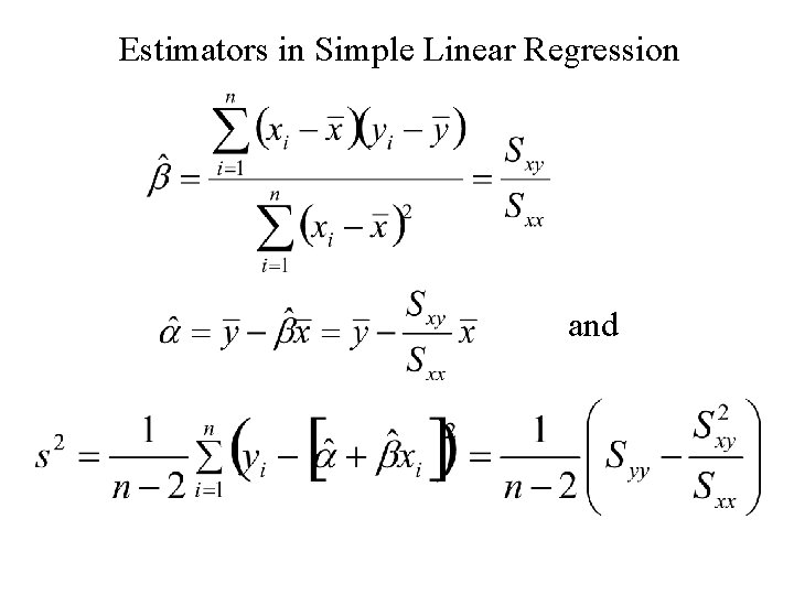
Estimators in Simple Linear Regression and

Sampling distributions of the estimators

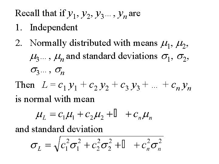
Recall that if y 1, y 2, y 3…, yn are 1. Independent 2. Normally distributed with means m 1, m 2, m 3…, mn and standard deviations s 1, s 2, s 3…, sn Then L = c 1 y 1 + c 2 y 2 + c 3 y 3 + … + cn yn is normal with mean and standard deviation

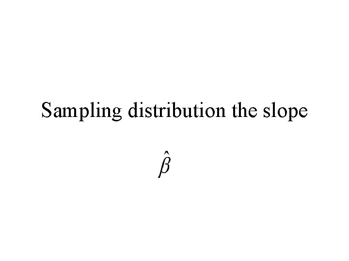
Sampling distribution the slope

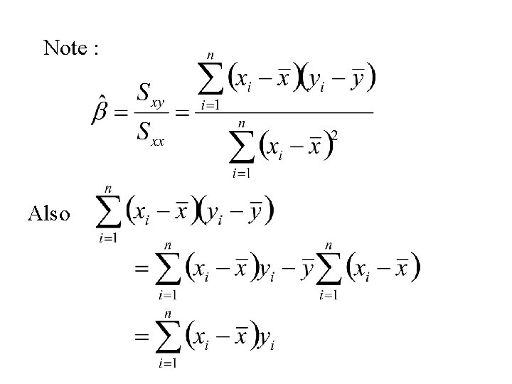
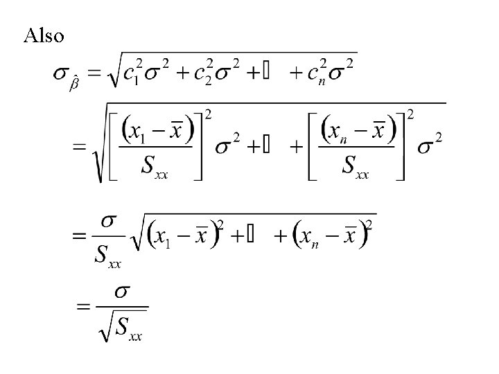
Note : Also

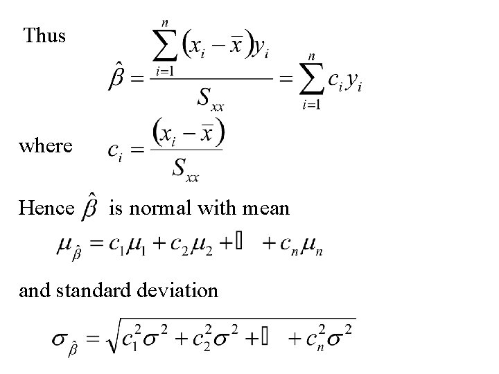
Thus where Hence is normal with mean and standard deviation

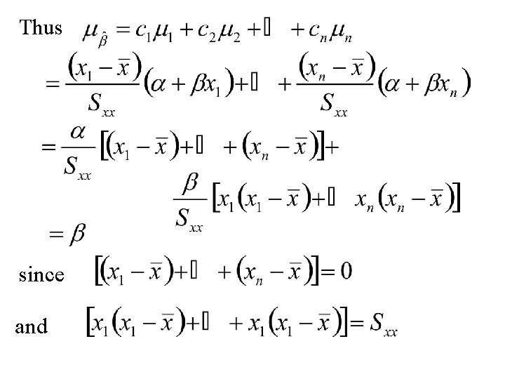
Thus since and

Also

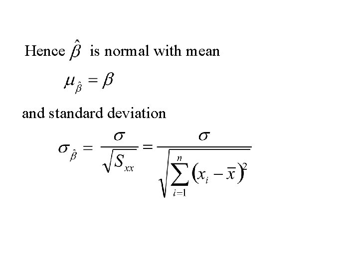
Hence is normal with mean and standard deviation

Sampling distribution of the intercept

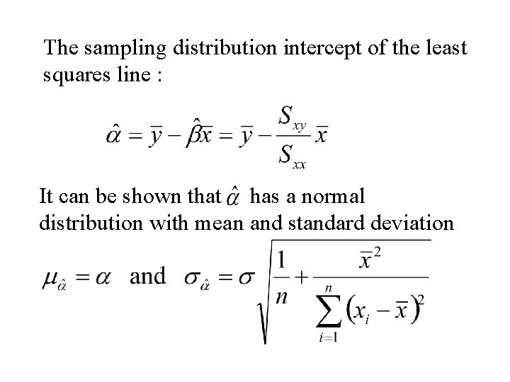
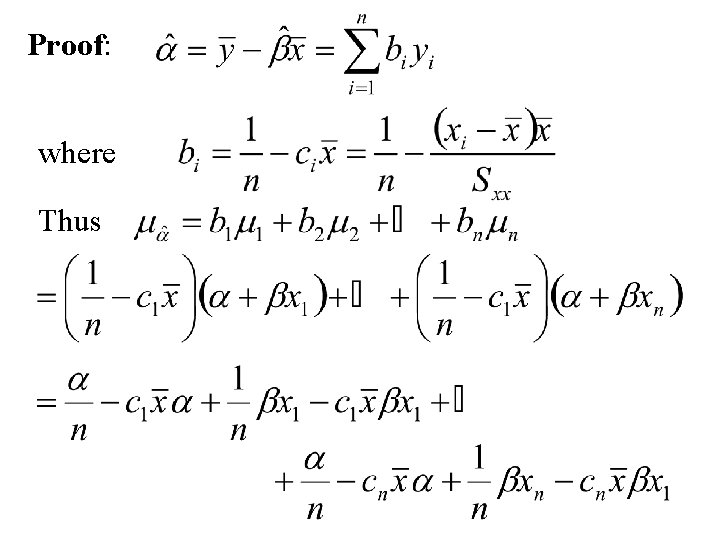
The sampling distribution intercept of the least squares line : It can be shown that has a normal distribution with mean and standard deviation

Proof: where Thus

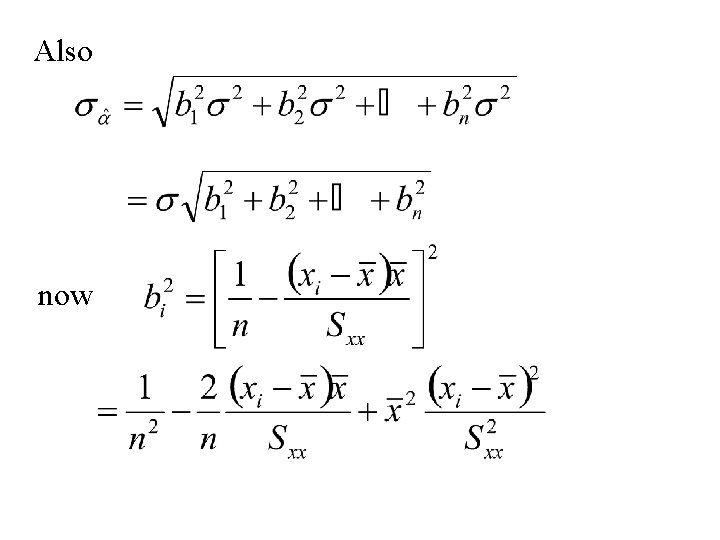
Also now

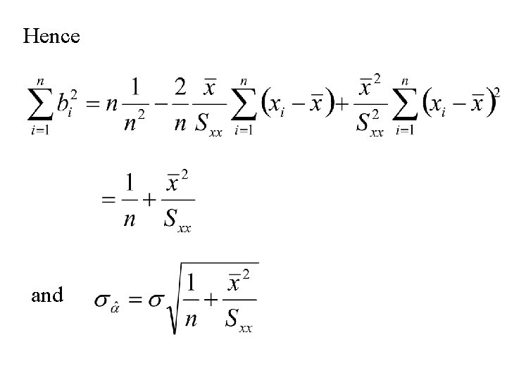
Hence and

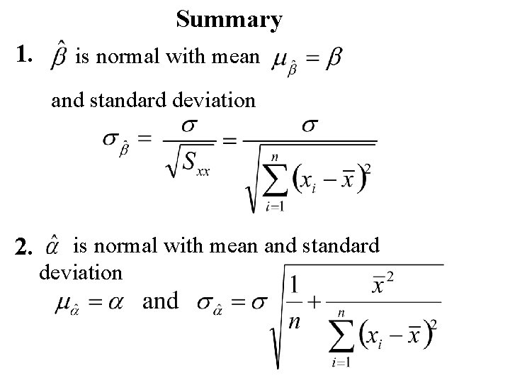
Summary 1. is normal with mean and standard deviation 2. is normal with mean and standard deviation

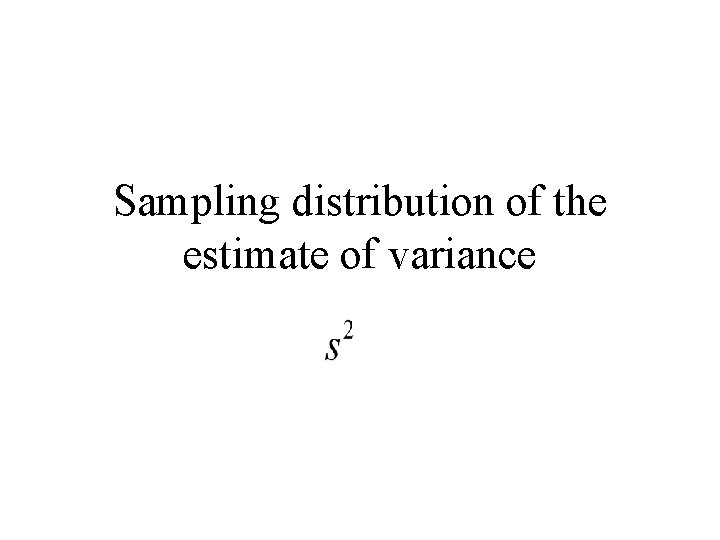
Sampling distribution of the estimate of variance

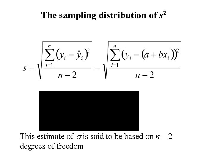
The sampling distribution of s 2 This estimate of s is said to be based on n – 2 degrees of freedom

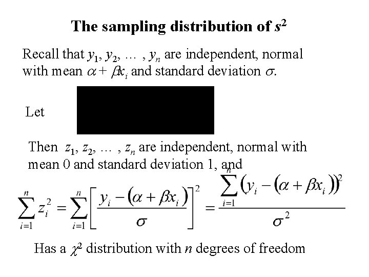
The sampling distribution of s 2 Recall that y 1, y 2, … , yn are independent, normal with mean a + bxi and standard deviation s. Let Then z 1, z 2, … , zn are independent, normal with mean 0 and standard deviation 1, and Has a c 2 distribution with n degrees of freedom

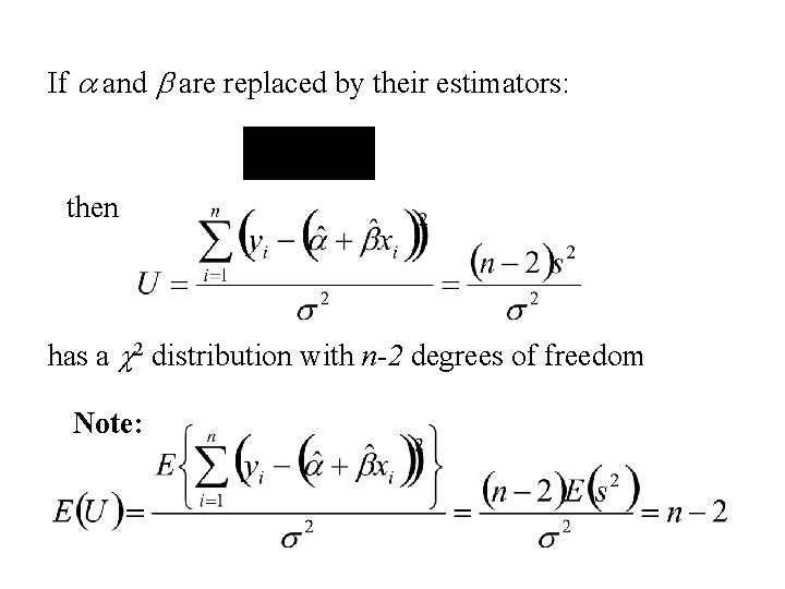
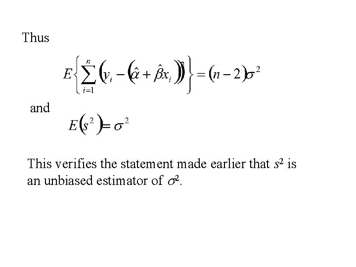
If a and b are replaced by their estimators: then has a c 2 distribution with n-2 degrees of freedom Note:

Thus and This verifies the statement made earlier that s 2 is an unbiased estimator of s 2.

Summary 1. is normal with mean and standard deviation 2. is normal with mean and standard deviation

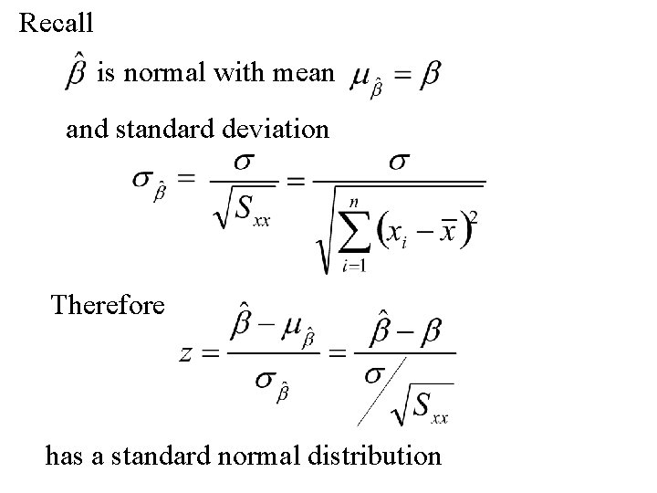
Recall is normal with mean and standard deviation Therefore has a standard normal distribution

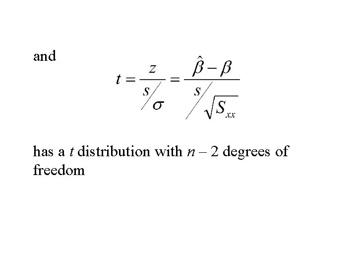
and has a t distribution with n – 2 degrees of freedom

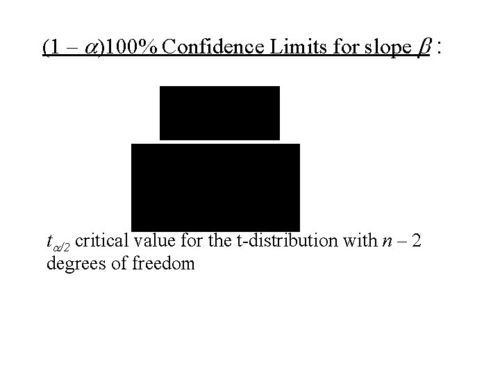
(1 – a)100% Confidence Limits for slope b : ta/2 critical value for the t-distribution with n – 2 degrees of freedom

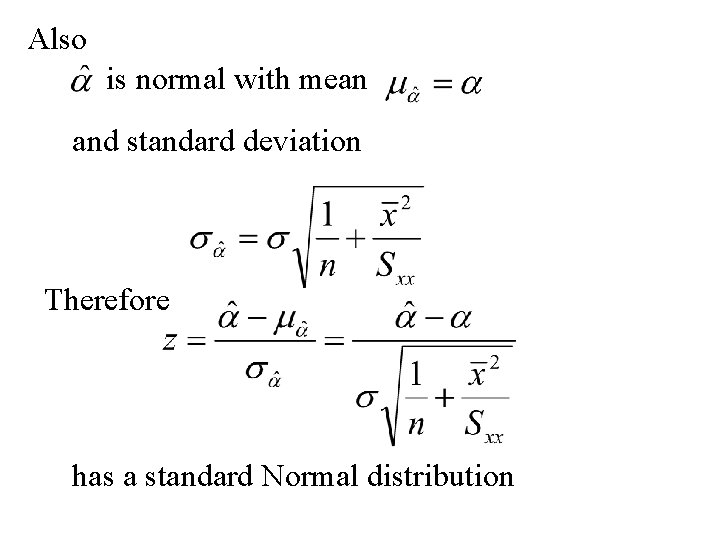
Also is normal with mean and standard deviation Therefore has a standard Normal distribution

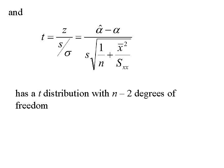
and has a t distribution with n – 2 degrees of freedom

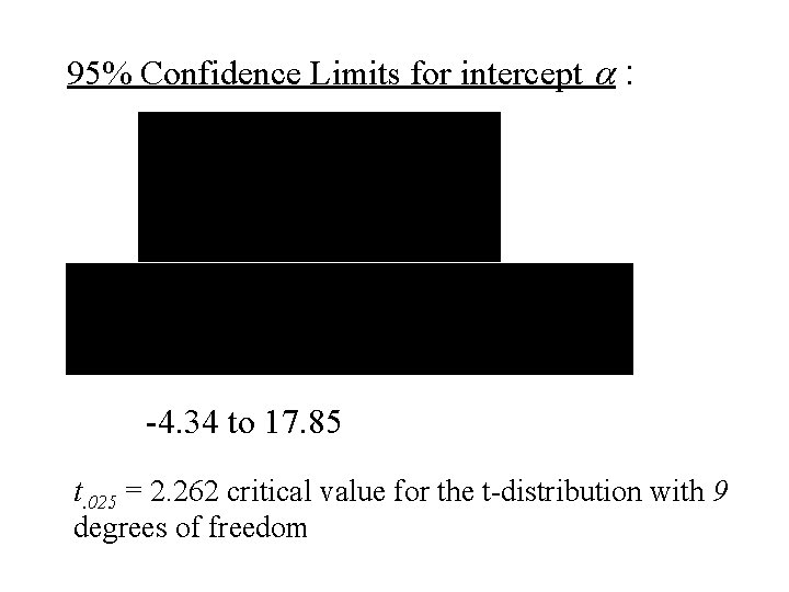
(1 – a)100% Confidence Limits for intercept a : ta/2 critical value for the t-distribution with n – 2 degrees of freedom

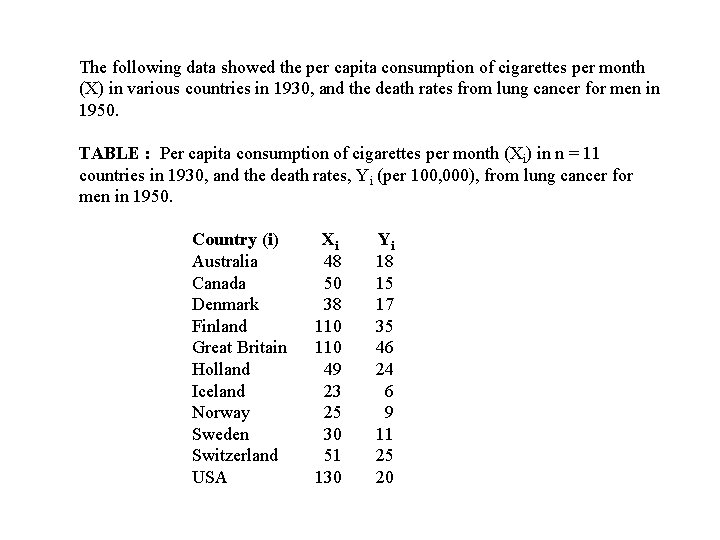
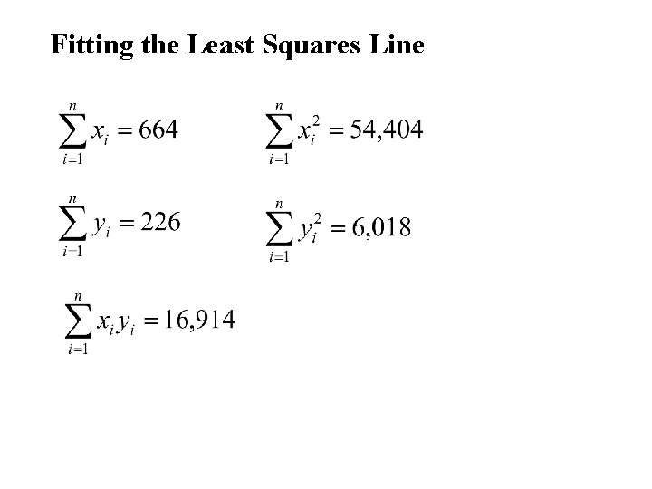
The following data showed the per capita consumption of cigarettes per month (X) in various countries in 1930, and the death rates from lung cancer for men in 1950. TABLE : Per capita consumption of cigarettes per month (Xi) in n = 11 countries in 1930, and the death rates, Yi (per 100, 000), from lung cancer for men in 1950. Country (i) Xi Yi Australia 48 18 Canada 50 15 Denmark 38 17 Finland 110 35 Great Britain 110 46 Holland 49 24 Iceland 23 6 Norway 25 9 Sweden 30 11 Switzerland 51 25 USA 130 20

Fitting the Least Squares Line

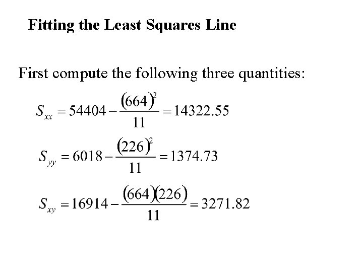
Fitting the Least Squares Line First compute the following three quantities:

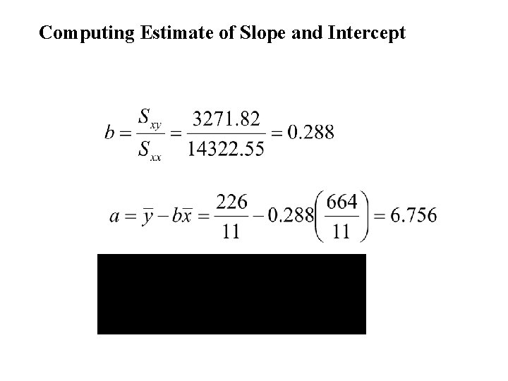
Computing Estimate of Slope and Intercept

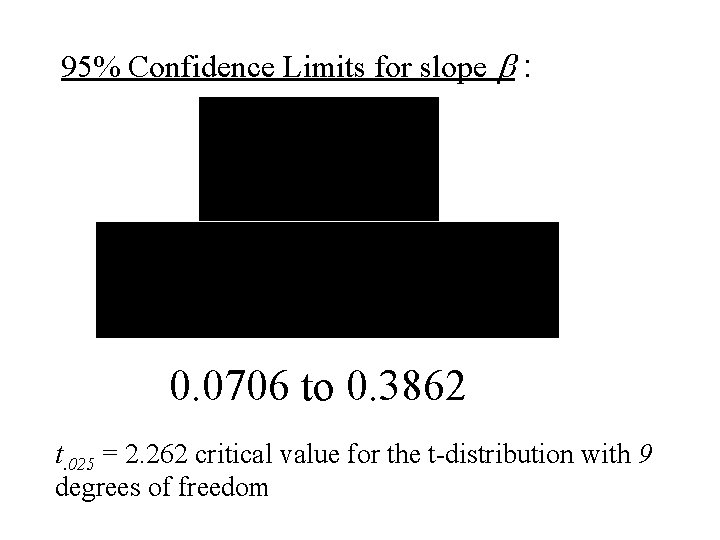
95% Confidence Limits for slope b : 0. 0706 to 0. 3862 t. 025 = 2. 262 critical value for the t-distribution with 9 degrees of freedom

95% Confidence Limits for intercept a : -4. 34 to 17. 85 t. 025 = 2. 262 critical value for the t-distribution with 9 degrees of freedom

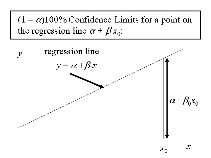
(1 – a)100% Confidence Limits for a point on the regression line a + b x 0: y regression line y = a +b 0 x 0 x

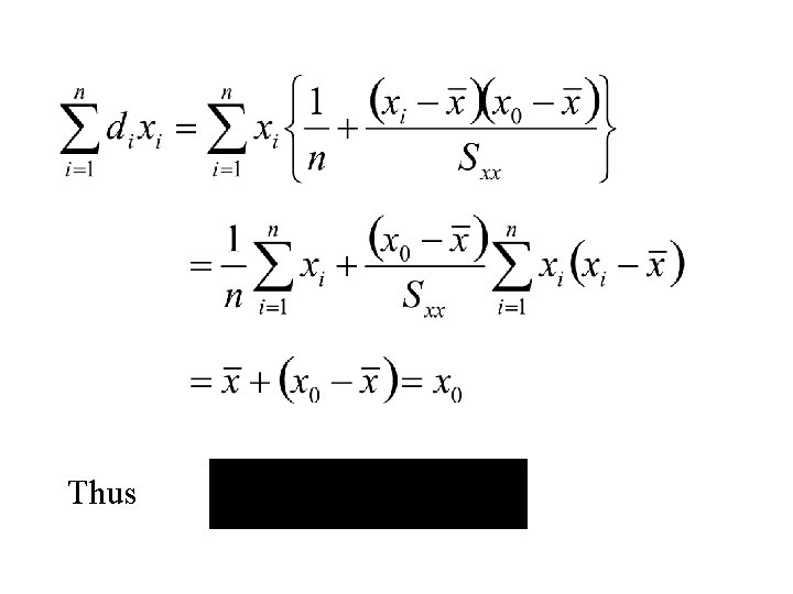
Let then and

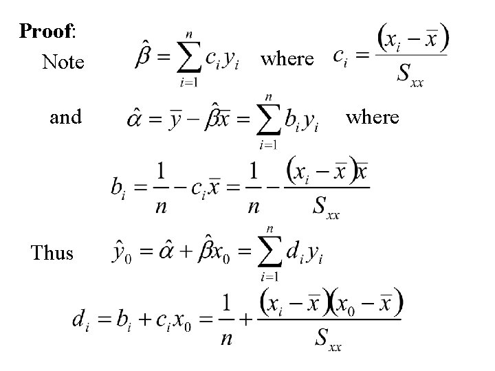
Proof: Note and Thus where

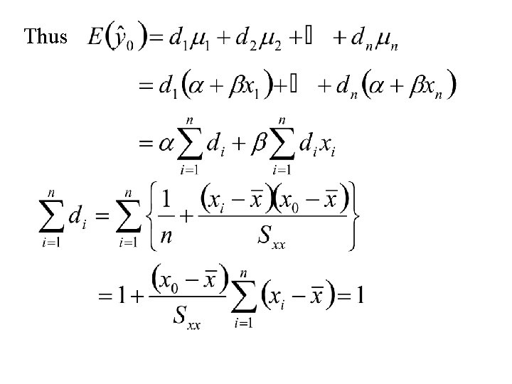
Thus

Thus

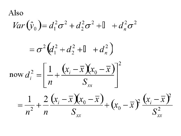
Also now

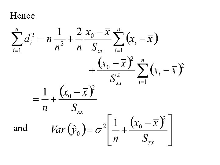
Hence and

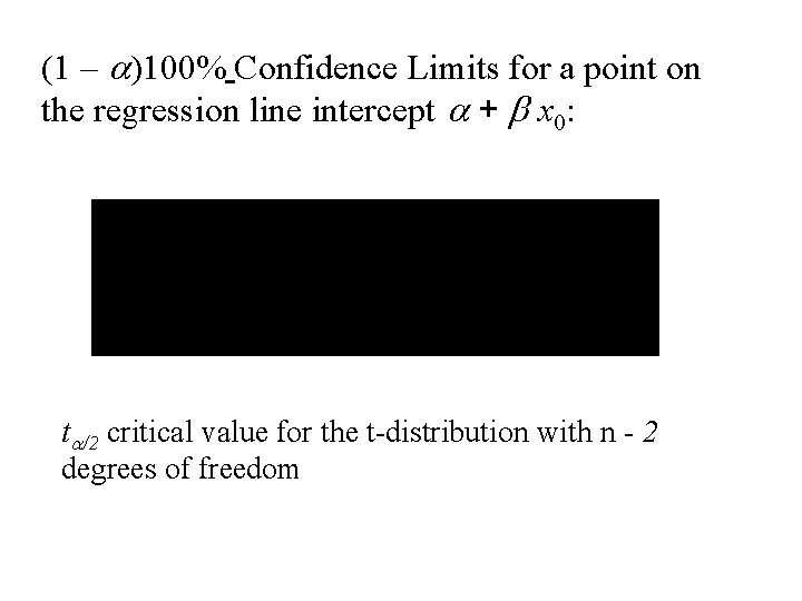
(1 – a)100% Confidence Limits for a point on the regression line intercept a + b x 0: ta/2 critical value for the t-distribution with n - 2 degrees of freedom

Prediction In linear regression model

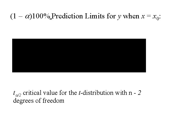
(1 – a)100% Prediction Limits for y when x = x 0: ta/2 critical value for the t-distribution with n - 2 degrees of freedom