The science of climate and atmospheric changes Due

The science of climate and atmospheric changes

Due to Natural Occurrence? Assumption of Linearity? • Increase of 317, 760, 00 per year • For every 17, 543, 859, 600 we see a 1 deg C increase • About 55 years for 1 deg C. • If 55 years is 1 degree, then 1375 years is 25 degrees • Therefore 13, 000 years is about 236 degrees

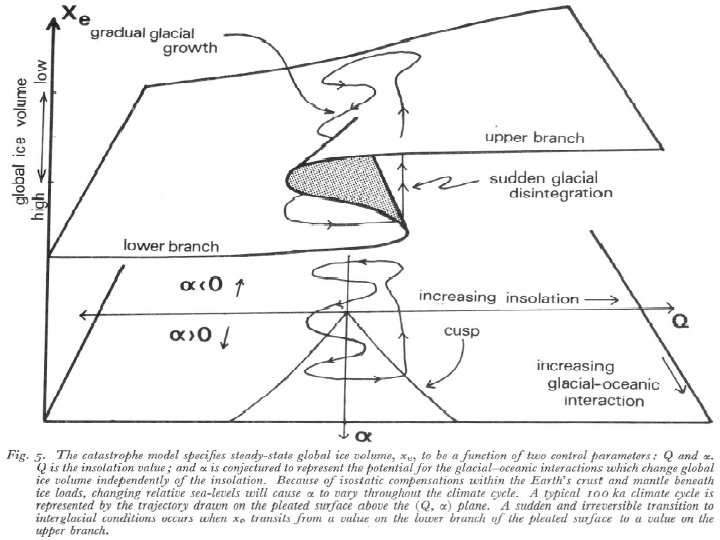
Figure X. XX The catastrophe model demonstrates a steady state behavior for a determined time interval. For all practical purposes, this is a linear system and therefore it is relatively predictable. As the values approach the lip of the cusp from the lower state, no change in the rate of change is meaningful. Before entry to the cusp, temperature actually slows due to the energy required to change state. Not all ice will melt at the same time therefore there will be a gradual reduction in the rate of change because of the additional solar energy needed to do the work required to change state of ice to water. PDF(Zdep) =�* exp(A * zasy 4 + B * dep 3 + C * asy 2 * zbif + D * zdep * zasy) The sudden “jump” that characterizes the cusp catastrophe model. It requires an additional 144 Btu to melt one pound of ice to one pound of water at 32 degrees F at atmospheric pressure. Therefore, depending on how many pounds of ice exist, temperature change will stop at 32 while a change of state takes place.

Carbon is Different than Regenerative and Absorptive Capacity Source: Joseph J Jacobsen (2011)

World Carbon Emission • Last year, all the world's nations combined pumped nearly 38. 2 billion tons of carbon dioxide into the air from the burning of fossil fuels such as coal and oil, according to new international calculations on global emissions published in the journal Nature Climate Change. That's about a billion tons more than the previous year. • The total amounts to more than 2. 4 million pounds of carbon dioxide released into the air every second.

Normal Variability CO 2 over a million years (blended cores) 400, 000 350, 000 300, 000 CO 2 (ppmv) 250, 000 200, 000 150, 000 100, 000 50, 000 1 42 83 124 165 206 247 288 329 370 411 452 493 534 575 616 657 698 739 780 821 862 903 944 985 10261067 Time in thousands of years starting in 1958 and working back - annual observations

Carbon • Global carbon emissions from man-made sources more than tripled from 1950 to 2000 and they continue to increase at a faster rate today. • From 1990 to 1999, global emissions increased at a rate of 1. 1% annually, to 3% after 1999. • This jump represents an increase to 28. 2 billion metric tons in 2005. • Reliable scientific estimates indicate that the tonnage will continue to climb to 33. 9 (B) in 2015 with further increases to 42. 9 (B) by 2030.

Emissions attributable to buildings found in the US from 1980 through 2030 Carbon Emissions of US Buildings (1, 000 Metric Tons) 1000 900 CO 2 800 885, 4 R 2 = 0, 9889 819, 4 760, 4 716, 4 667, 1 630, 3 593, 5 700 600 500 400 1970 427, 1 470, 9 1990 2010 Year 2030 2050

Source: Joseph J Jacobsen (2011)

Wouldn’t it be great if we could suddenly double the economy? Economic growth has been the national goal for most nations for better than 100 years and it has been working to produce results that have steadily lifted standards of living to miraculous heights. The US economy doubled from 1933 ($511 billion) to 1942 from 1942 to 1962 from 1962 to 1979 and from 1979 to 2004 while the population of the US has gone from 131 to 300 million. Over the long run, GDP shows no signs of slowing down in the future. The basic underpinning of the free economy is that we are all self interested and as a result we work harder to grow our personal wealth and as a result of millions of people working harder, the economy grows. Has this economic concept reached the end of its useful life?

Global CO 2 in PPM from 1959 to 2010 400 CO 2 ppm 380 360 340 R 2 = 0, 987 320 300 1949 1959 1969 1979 1989 Year 1999 2009 2019

Source: Joseph J Jacobsen (2011)

Source: Joseph J Jacobsen (2011)

Source: Joseph J Jacobsen (2011)

Due to Natural Occurrence? Assumption of Linearity? • Increase of 317, 760, 00 per year • For every 17, 543, 859, 600 we see a 1 deg C increase • About 55 years for 1 deg C. • If 55 years is 1 degree, then 1375 years is 25 degrees • Therefore 13, 000 years is about 236 degrees

Reporting Carbon Footprint: the classifications • Scope 1 – all direct greenhouse gas emissions • Scope 2 – Indirect greenhouse gas emissions from consumption of electricity, heat or steam • Scope 3 – Other indirect emissions, such as the extraction and production of purchased materials and fuels, transport related activities in vehicles not owned by the business, electricity related operations not covered in scope 2, outsourced operations, supplier chains and operations and waste disposal processes.

Carbon Statistics Per Product Per 1000 Sq/Ft Person Reduction Percent Offset Goal Emissions: Scope 1 Emissions: Scope 2 Emissions: Scope 3 Emissions: total Simple emissions inventory table that can be easily inserted into a report or presentation. CO 2 per product, per 1000 square feet and person are entered into the fields at the appropriate emission scope.

Energy Value CO 2 (Kgs. ) CO 2 (Lbs. ) Btu 1 gallon of gas 8. 9 19. 62 114, 100 1 pound of coal 1 1. 3 2. 86 14, 000 1 ton of coal 2, 594. 55 5, 720 28, 000 1, 000 cubic feet of natural gas 54. 7 120. 59 100, 000 1 k. Wh of electricity 1. 34 3, 412 . 61

• Useful Ratios Btu per degree day is the definitive measure for commercial buildings. Btu/DD • As time moves on, we should see a decrease in the amount of Btu it takes to offset the outside temperature. This is the true measure of the physical plants efficiency. Watts per square foot is the definitive measure for lighting efficiency for a commercial building. It is important to measure performance using repeatable and valid measures • The first ratio is an account of how much value every unit of CO 2 brings relative to a fuel source. In the instance of renewable energy, where no CO 2 results from every unit of useful output, the ratio is some value output divided by zero and is undefined so renewable energy is in a category that only measures output in real numbers. The ratio that I refer to as the Jacobsen usefulness/CO 2 ratio is used to measure the internality/externality value of a fuel. The resulting value derived from this division is the overall usefulness (Btu) per unit of negative externality, CO 2. After identifying the baseline, on a spreadsheet, this number should increase over time by decreasing CO 2 and/or increasing efficiency of energy using systems. Btu/CO 2 • The next ratio is the Jacobsen cost of energy ratio and it measures the energy per economic cost (dollars) of a fuel in Btu (equation 2). Btu/$ • After identifying the baseline, on a spreadsheet, this number should increase over time by decreasing costs and/or increasing output of energy systems per unit of expense.

The total reduction in dollars of incandescent lighting operations would be $44, 000 over a 5 year period if we continue to use the incandescent lamps. The total (5 year) carbon emissions for the incandescent option is 148, 260 pounds over 5 years. Incandescent Lamp 1 2 3 4 5 Total Incandescent purchase 1000 1000 $5000 Incandescent labor 3000 3000 $15000 Incandescent energy 4800 4800 $24000 Emissions 29, 652 29, 652 148, 260 Total cost of incandescent option 8800 8800 $44, 000

Total dollars, energy and carbon emissions are captured on a single table. The carbon emission of the CFL lighting operations would be 5, 360 pounds over the 5 year period. CFL Lamp 1 2 3 4 5 Total CFL purchase 4, 000 0 0 $4, 000 CFL labor 3, 000 0 0 $3, 000 CFL energy 800 800 800 $4, 000 CFL carbon emissions 1, 072 1, 072 5, 360 lbs. Total Cost $11, 000

Net Electricity Generation by Type and Country (2007) 4, 156. 7 represents 4, 156, 700, 000. k. Wh = kilowatt hours, world total is 18, 778, 700, 000. k. Wh = kilowatt hours 4 500, 00 4 000, 00 3 500, 00 3 000, 00 2 500, 00 2 000, 00 1 500, 00 1 000, 00 500, 00 Un i te d St at es Ch in a Ja pa n Ru ss ia In di Ca a na Ge da rm an Fr y an ce Ko Br Un rea azil ite , So d Ki uth ng do m Ita ly Sp ai M n So ex ut ico h Af ric a 0, 00

Aside from living systems, energy is the single most important aspect of the economic world. This is because energy has the capacity to do work. That is, energy is the work which may be stored up in a substance in such a way that it may be used on demand.

Heating Value of Fuel The amount of heat expressed in B. T. U. produced by the complete combustion of 1 pound of any fuel is called the heating value of that fuel. It is also sometimes called the heat of combustion. For instance, 1 pound of hydrogen burned to water will liberate 62, 000 B. T. U. Therefore, the heating value of hydrogen is 62, 000 B. T. U. If we know the percentage by weight of the elements composing a fuel, we can calculate approximately the heating value of that fuel by the following formula: B. T. U. = 14, 600 C + 62, 000 (H – O/8) In which, C = amount of carbon in 1 pound of fuel, H = amount of hydrogen in 1 pound of fuel, O = amount of oxygen in 1 pound of fuel. The term O/8 is subtracted because oxygen contained in hydrogen compounds has no heating value and since it is already combined with a portion of the hydrogen of these compounds, it reduces the heating value of the fuel somewhat. The factor 8 is used because oxygen combines with hydrogen in the ratio of 1: 8.

Carbon Emissions Attributable to Scope 1 Fossil Fuel Combustion vs. Scope 2 Electricity US Buildings Carbon Emissions (1, 000 Metric Tons) 1000 900 800 CO 2 Emissions 700 600 500 Fossil 400 Electricity 300 Total 200 100 0 1970 1980 1990 2000 Year 2010 2020 2030 2040

Buildings Sector Accounts for About 40% of U. S. Energy, 72% of Electricity, 34% of Natural Gas, 38% of Carbon, 18% of NOx, and 55% of SO 2 Emissions. Total U. S. Consumption in 2005 was 100 Quads Building Sector construction and renovation accounts for 9% of GDP and employs 8 million people. Energy utility bills total $390 B each year. Source: Buildings Energy Data Book, September 2008, Tables 1. 1. 3, 1. 1. 6, 3. 1. 1, 3. 3. 1, 4. 1. 5, 5. 1. 2, 5. 3. 1

Energy consumed CO 2 Emissions Utility costs Commercial Building Energy Consumption Impact 25 QUADS 1. 4 Gigatons $227 Billion Current Inventory 5 M Buildings 18 QUADS 1. 1 Gigatons $170 Billion 2011 Source: Buildings Energy Data Book Projected Years 2030

Commercial Building Energy Impact • An analysis of building commissioning practices found deficiencies in design, construction, equipment operation, and deferred maintenance that compromised indoor air quality and comfort, cause unnecessary elevated energy use and/or under-performing energyefficiency strategies. • Whole-building energy savings of 15% with median payback times of 0. 7 years can be realized. • There is nothing greener than a well run facility.

Potential Savings/Emissions Impact $280 $260 If started in 2010, an average of $29 B savings and a reduction of 191 M tons CO 2 emissions per year can potentially be realized Utility Costs - Billion $240 $220 $200 Linear(Projected Utility Costs) $180 Linear(Projected Savings) $160 $140 $120 $100 2015 Source: Buildings Energy Data Book, October 2009 2020 2025 2030