The Schrdinger Equation The first step in the

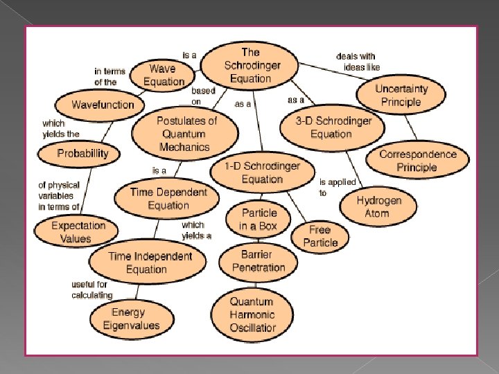
The Schrödinger Equation The first step in the development of a logically consistent theory of non-relativistic quantum mechanics, wave-like behavior of a quantum particle – the Schrödinger Equation.

The Schrödinger Equation � In Quantum Mechanics/Quantum Physics, particles have wavelike properties, and a particular wave equation, the Schrödinger Equation – governs how these wave behave.

Schrödinger Equation � WAVES - Sinusoidal waves Very often in classical physics, and invariably in quantum physics, sinusoidal travelling waves are represented by complex exponential Function of the form: where; (x, t) = A ei(kx- t) = cos (kx- t) + i sin (kx- t) In quantum physics, the use of complex numbers is not an option-because complex exponential function provides a natural description of a de Broglie wave.

Schrödinger Equation � The DERIVATION of Schrödinger equation. The starting point will be the classical non-relativistic expression for the energy of a particle, which is the sum of the K. E and P. E. Assume in 1 D of a function only in x-direction: E = K. E + P. E = K + V = ½ mv 2 + V(x) = p 2/2 m + V(x)……(1) We’ll now invoke de Broglie’s claim that all particles can be represented as waves with frequency and wavenumber k, and that E = ħ and p = ħ k. This turn the expression for the energy into: Im p ! t an t or …………………. . (2)

Schrödinger Equation � o A wave with frequency and wavenumber k can be written as usual as (x, t)=Aexp[i(kx- t)], for 3 D, replace x with vector r, which represented x, y, and z axis. But, let’s just deal with 1 D, we now note that: …………. (3) If we multiply the energy equation (2) by , and plug in these relation (3), we obtain: Time-dependent Schrödinger equation (TDSE)

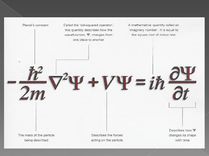
Schrödinger Equation � If we put the x and t arguments back in, the equation (TDSE) takes the form (in 1 D): The Schrödinger Equation (S. E) actually is not valid – so there’s certainly no way that we proved it. The quantum theory based on S. E is just a limiting theory of a more correct one, which happens to be Quantum Field Theory (unifies quantum mechanics with special relativity). � S. E doesn’t incorporate gravity. Eventually, there will be one theory that covers everything – but we definitely not there yet!. �

Schrödinger Equation

Schrödinger Equation Due to “i ” (i= (-1)) that appears in TDSE above, (x) is complex – contrast with waves in classical mechanics, the entire complex function now matters in quantum mechanics. V(x, t) is the classical potential. � As a wavefunction in exponential complex function, because it easier to work rather than trig. function. � Anything you want to measure: position, momentum, energy, etc – will always turn out to be a real quantity. � By ignoring all limits, let’s just accept S. E as valid. In 3 -D problem, S. E written as: � Laplacian:

Schrödinger Equation A WAVE EQUATION FOR A FREE PARTICLE q For a freely moving non-relativistic particle by considering the properties of the de Broglie waves describing the particle. q A particle with momentum p has a de Broglie wavelength given by =h/p, this implies that de Broglie wave with wavenumber k = 2 / describes a particle with momentum p=ħk, ħ = h/2. q By assuming that de Broglie wave packet with a range of wavenumber between k-∆k and k+∆k describes a particle with an uncertain momentum; ∆p≈ ħ∆k Also, assume that the length of wave packet is a measure of ∆x, the uncertainty in the position of the particle, thus ∆x ≈ 2 /∆k Multiply both uncertainties, we obtain: ∆x ∆p ≈ h Good agreement with H. U. P.

Schrödinger Equation � The de Broglie waves describing a freely moving quantum particle of mass m: This relation obtained by integrating d /dk = ħk/m by setting the constant of integration to zero – gives rise to no observable consequences in non-relativistic quantum mechanics. � For a free particle moving in 1 D, it has the form: � And the solution of the above eq. is (x, t)=Aexp[i(kx- t)]

Schrödinger Equation The interaction of a non-relativistic particle can usually be described in terms of a potential energy field V(r). � For example, an electron in a H atom can be thought of as moving in the potential energy field, V (r) = e 2/4 0 r of a nucleus. � In Classical Mechanics, this field implies that an electron at a distance r from the nucleus experiences an attractive force of magnitude e 2/4 0 r 2. � In QM, it implies that the wave function for the electron is not simple free-particle wave equation – must have additional V(r) as a total energies of K. E and P. E (Hamiltonian). �

Schrödinger Equation

Position & Momentum probabilities

Position & Momentum probabilities � Comparing to the double slit experiment.

Interference pattern Position & Momentum probabilities

Position & Momentum probabilities

Position & Momentum probabilities

Position & Momentum probabilities

Schrödinger Equation: Solving the Equation. From TDSE, we already know the solution, of course, using (x, t)=Aexp[i(kx- t)], but let’s pretend that we don’t know this. � As always, we’ll guess an exponential solution, our guess is (x, t)=exp[-i t]f(x), and subst. into TDSE, then: �

Schrödinger Equation: Solving the Equation. This is called the time-independent Schrödinger Equation (TISE). This TISE is appropriate when V is independent of time. Otherwise, you use the full TDSE. � E – particle energy. �

Schrödinger Equation: Solving the Equation. � - Constant Potential The simplest example is where we have a constant potential V(x) = V 0 in the given region. Plugging (x)=A exp(ikx) into TISE, then gives: -only +ve value of k, and k is constant (wavenumber); its real/imaginary nature depends on the relation between E and V 0.

! t n Schrödinger Equation: Solving the rta po Equation. Im � • • If E > V 0; then k is real, so we have oscillatory solutions: (x)=A exp (ikx) + B exp (-ikx) If E < V 0; then k is imaginary, so we have exponentially growing or decaying solutions. If we let = |k| = (2 m[V 0 –E)/ħ, then (x) takes the form: (x)=A exp ( x) + B exp ( x) If E = V 0 ; guessing an exponential function doesn’t work, from TISE, this conditions implies 2 / x 2 = 0, so is LINEAR function, where (x)=A x + B

Schrödinger Equation: Solving the Equation. � � In all of these cases, the full wavefunction (including the time dependence) for a particle with a specific value of E is given by We use letter to stand for two different functions here. Any general wavefunction is built up from a superposition of the states above with different values of E, just as the general motion of a string is built of from various normal modes with different frequencies .

Relation between Quantum and Classical Mechanics.

Relation between Quantum and Classical Mechanics.

Relation between Quantum and Classical Mechanics.

Relation between Quantum and Classical Mechanics.

Relation between Quantum and Classical Mechanics. The other theorem – Ehrenfest theorem.

Relation between Quantum and Classical Mechanics.

Relation between Quantum and Classical Mechanics.

Relation between Quantum and Classical Mechanics.

Relation between Quantum and Classical Mechanics.

Relation between Quantum and Classical Mechanics. Further reading: WKB approximation….

Relation between Quantum and Classical Mechanics.

Relation between Quantum and Classical Mechanics.

For further understanding � V 1 � V 2