The Roy Model The Roy Model Village economy

The Roy Model

The Roy Model • Village economy. • There are two occupations: – Hunter – Fisherman • Fish and rabbits are completely homogeneous. • No uncertainty in the number that you catch. • Hunting is “easier” (you just set traps).

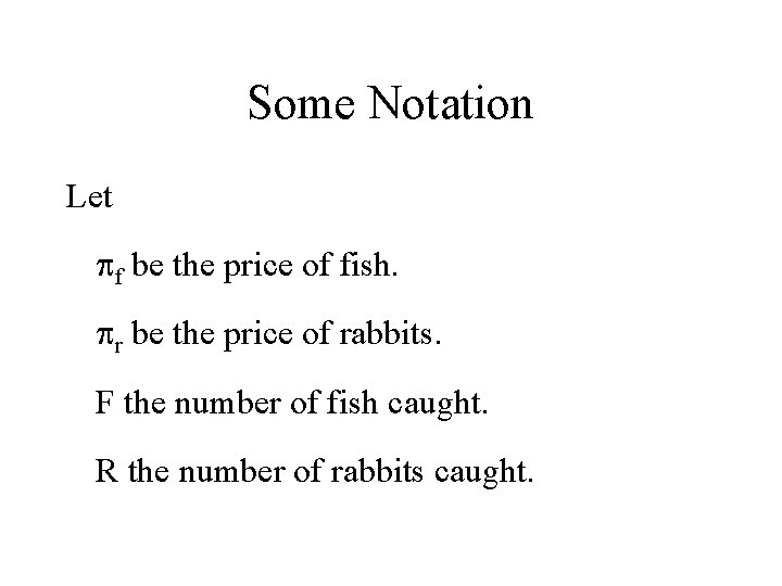
Some Notation Let pf be the price of fish. pr be the price of rabbits. F the number of fish caught. R the number of rabbits caught.

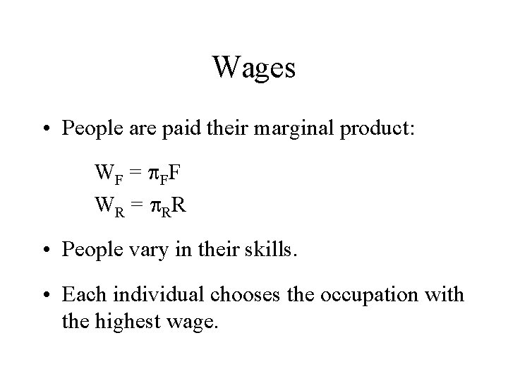
Wages • People are paid their marginal product: W F = p FF WR = p. RR • People vary in their skills. • Each individual chooses the occupation with the highest wage.

Key Questions • Do the best hunters hunt? • Do the best fishermen fish? It turns out the answer depends on the variance of skill (nothing else!). – Whichever happens to have the largest variance in logs will tend to have more sorting. – In particular, demand doesn’t matter.

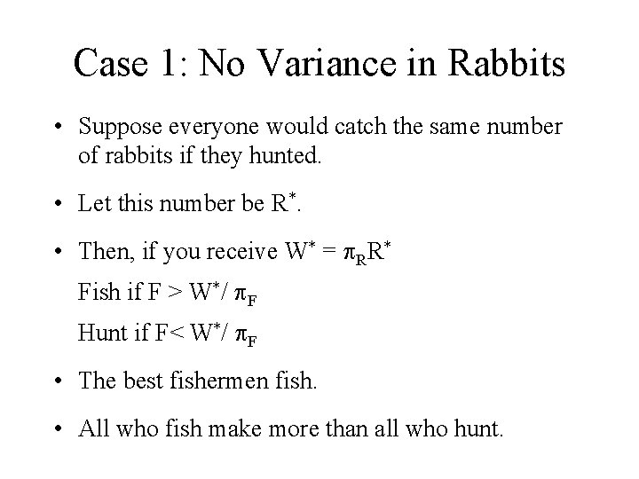
Case 1: No Variance in Rabbits • Suppose everyone would catch the same number of rabbits if they hunted. • Let this number be R*. • Then, if you receive W* = p. RR* Fish if F > W*/ p. F Hunt if F< W*/ p. F • The best fishermen fish. • All who fish make more than all who hunt.

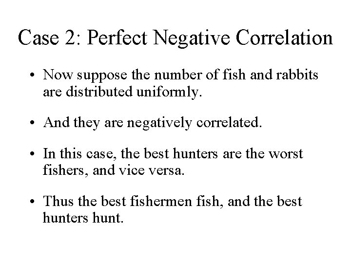
Case 2: Perfect Negative Correlation • Now suppose the number of fish and rabbits are distributed uniformly. • And they are negatively correlated. • In this case, the best hunters are the worst fishers, and vice versa. • Thus the best fishermen fish, and the best hunters hunt.

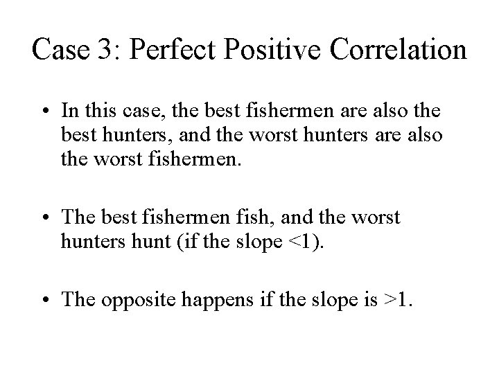
Case 3: Perfect Positive Correlation • In this case, the best fishermen are also the best hunters, and the worst hunters are also the worst fishermen. • The best fishermen fish, and the worst hunters hunt (if the slope <1). • The opposite happens if the slope is >1.

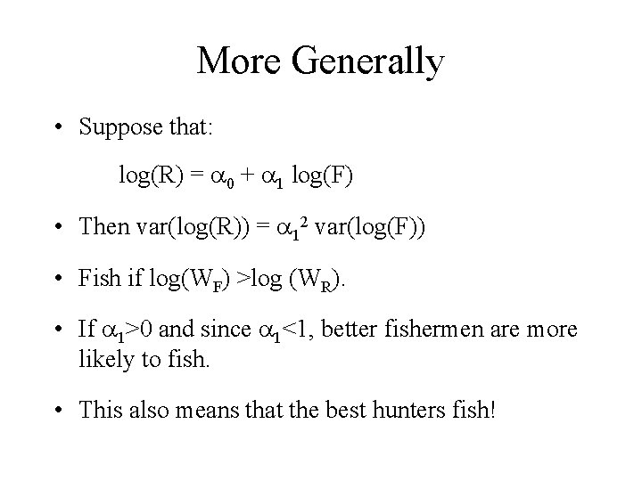
More Generally • Suppose that: log(R) = a 0 + a 1 log(F) • Then var(log(R)) = a 12 var(log(F)) • Fish if log(WF) >log (WR). • If a 1>0 and since a 1<1, better fishermen are more likely to fish. • This also means that the best hunters fish!

Negative Correlation • If a 1<0, better fishermen still fish. • But now the best hunters hunt.

Case 4: Log Normal Random Variables • Let’s try to think of this in other cases. • Assume that: (log(R), log(F)) N(m, S)

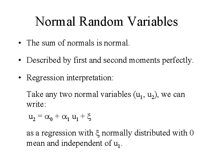
Normal Random Variables • The sum of normals is normal. • Described by first and second moments perfectly. • Regression interpretation: Take any two normal variables (u 1, u 2), we can write: u 2 = a 0 + a 1 u 1 + x as a regression with x normally distributed with 0 mean and independent of u 1.

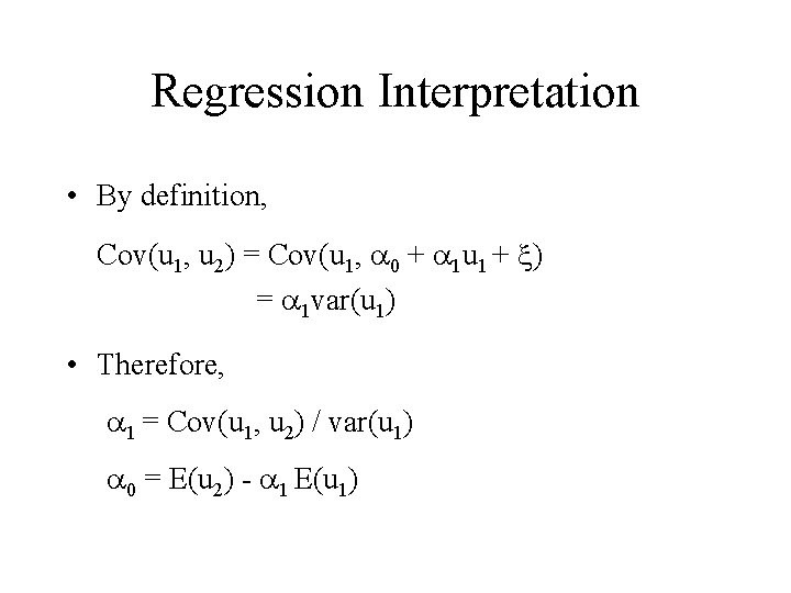
Regression Interpretation • By definition, Cov(u 1, u 2) = Cov(u 1, a 0 + a 1 u 1 + x) = a 1 var(u 1) • Therefore, a 1 = Cov(u 1, u 2) / var(u 1) a 0 = E(u 2) - a 1 E(u 1)

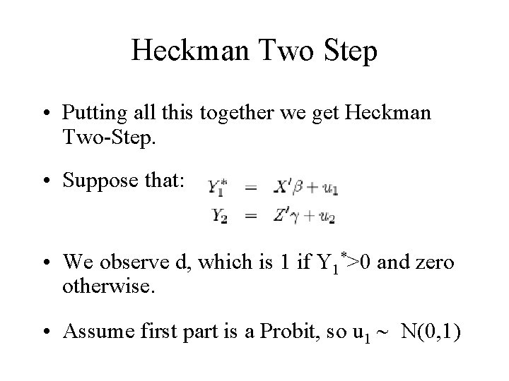
The Inverse Mills Ratio • If u N(0, 1), then E[u| u>k] = f(k) / (1 – F(k)) = l(-k) the inverse mills ratio.

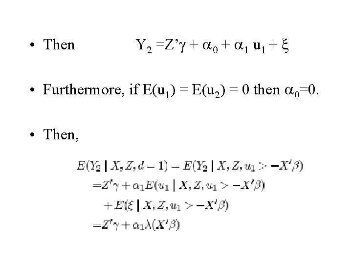
Heckman Two Step • Putting all this together we get Heckman Two-Step. • Suppose that: • We observe d, which is 1 if Y 1*>0 and zero otherwise. • Assume first part is a Probit, so u 1 N(0, 1)

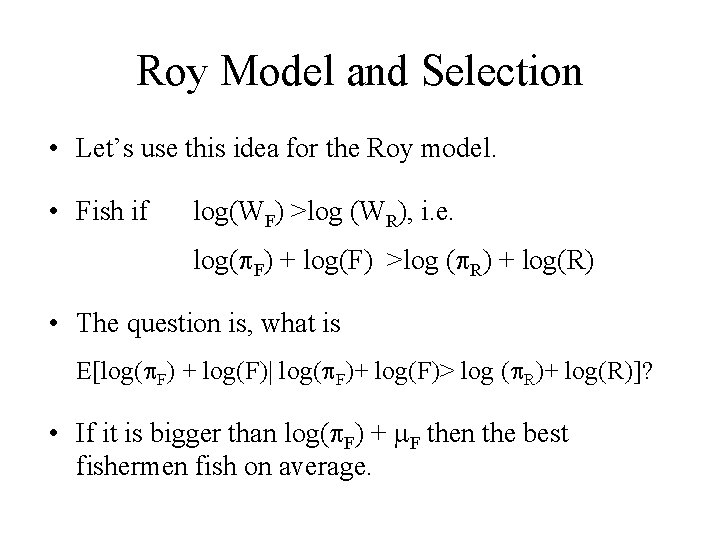
• Then Y 2 =Z’g + a 0 + a 1 u 1 + x • Furthermore, if E(u 1) = E(u 2) = 0 then a 0=0. • Then,

Roy Model and Selection • Let’s use this idea for the Roy model. • Fish if log(WF) >log (WR), i. e. log(p. F) + log(F) >log (p. R) + log(R) • The question is, what is E[log(p. F) + log(F)| log(p. F)+ log(F)> log (p. R)+ log(R)]? • If it is bigger than log(p. F) + m. F then the best fishermen fish on average.

Some Notation • Then,

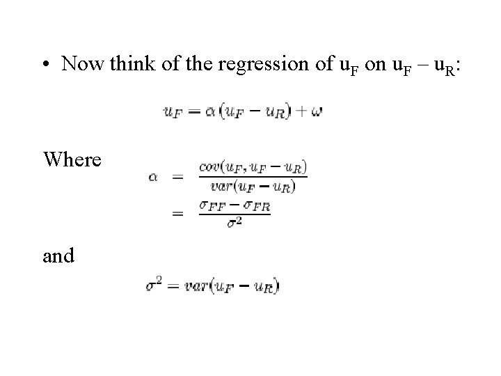
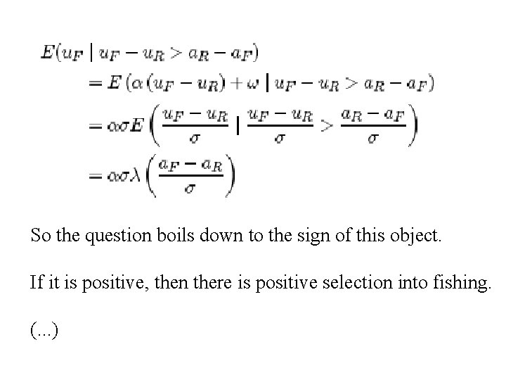
• Now think of the regression of u. F on u. F – u. R: Where and

So the question boils down to the sign of this object. If it is positive, then there is positive selection into fishing. (. . . )

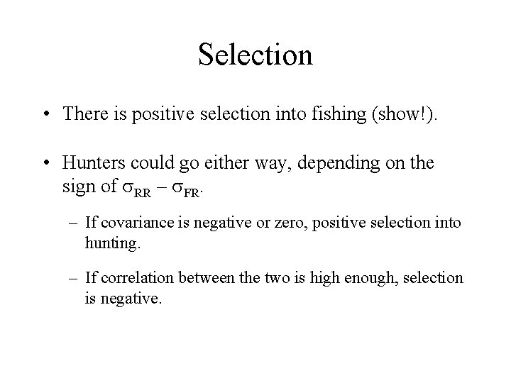
Selection • There is positive selection into fishing (show!). • Hunters could go either way, depending on the sign of s. RR – s. FR. – If covariance is negative or zero, positive selection into hunting. – If correlation between the two is high enough, selection is negative.

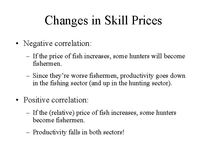
Changes in Skill Prices • Negative correlation: – If the price of fish increases, some hunters will become fishermen. – Since they’re worse fishermen, productivity goes down in the fishing sector (and up in the hunting sector). • Positive correlation: – If the (relative) price of fish increases, some hunters become fishermen. – Productivity falls in both sectors!

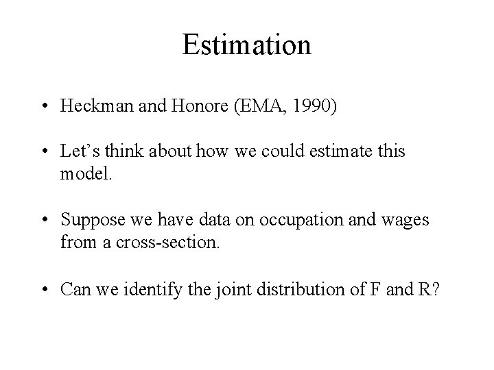
Estimation • Heckman and Honore (EMA, 1990) • Let’s think about how we could estimate this model. • Suppose we have data on occupation and wages from a cross-section. • Can we identify the joint distribution of F and R?

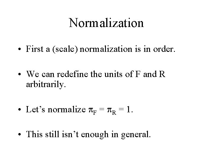
Normalization • First a (scale) normalization is in order. • We can redefine the units of F and R arbitrarily. • Let’s normalize p. F = p. R = 1. • This still isn’t enough in general.

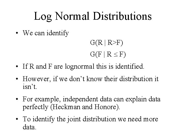
Log Normal Distributions • We can identify G(R | R>F) G(F | R F) • If R and F are lognormal this is identified. • However, if we don’t know their distribution it isn’t. • For example, independent data can explain data perfectly (Heckman and Honore). • To identify the joint distribution we need more data.

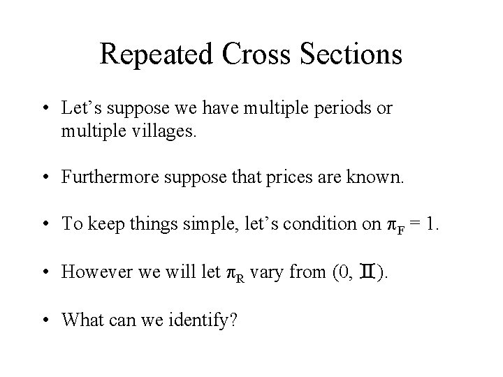
Repeated Cross Sections • Let’s suppose we have multiple periods or multiple villages. • Furthermore suppose that prices are known. • To keep things simple, let’s condition on p. F = 1. • However we will let p. R vary from (0, ). • What can we identify?

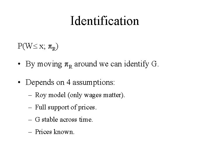
Identification P(W x; p. R) • By moving p. R around we can identify G. • Depends on 4 assumptions: – Roy model (only wages matter). – Full support of prices. – G stable across time. – Prices known.

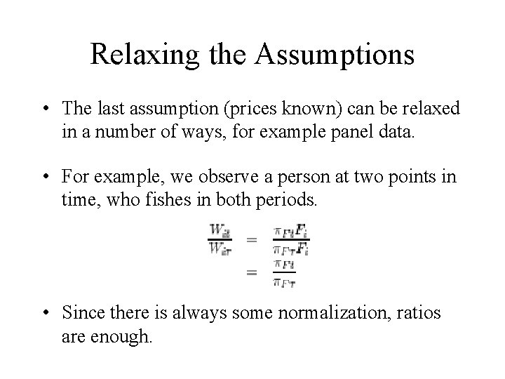
Relaxing the Assumptions • The last assumption (prices known) can be relaxed in a number of ways, for example panel data. • For example, we observe a person at two points in time, who fishes in both periods. • Since there is always some normalization, ratios are enough.

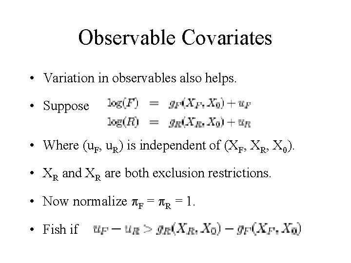
Observable Covariates • Variation in observables also helps. • Suppose • Where (u. F, u. R) is independent of (XF, XR, X 0). • XR and XR are both exclusion restrictions. • Now normalize p. F = p. R = 1. • Fish if

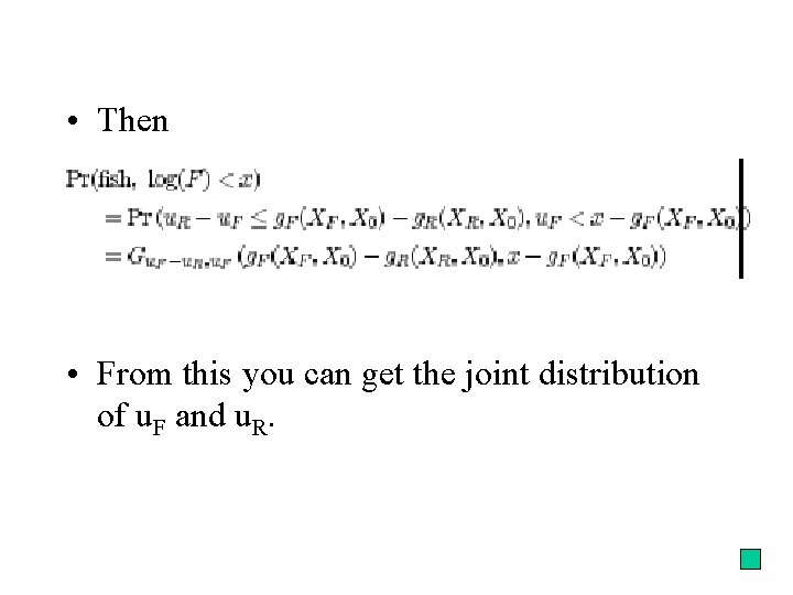
• Then • From this you can get the joint distribution of u. F and u. R.