The Role of Sensitivity Analysis of the Optimal

The Role of Sensitivity Analysis of the Optimal Solution • Is the optimal solution sensitive to changes in input parameters? • Possible reasons for asking this question: – Parameter values used were only best estimates. 1 – Dynamic environment may cause changes.

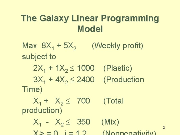
The Galaxy Linear Programming Model Max 8 X 1 + 5 X 2 (Weekly profit) subject to 2 X 1 + 1 X 2 £ 1000 (Plastic) 3 X 1 + 4 X 2 £ 2400 (Production Time) X 1 + X 2 £ 700 (Total production) X 1 - X 2 £ 350 (Mix) 2

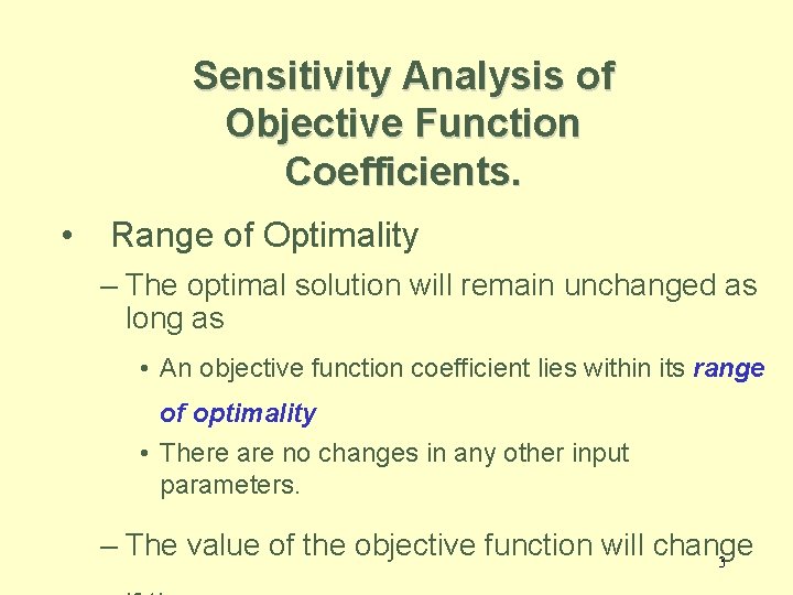
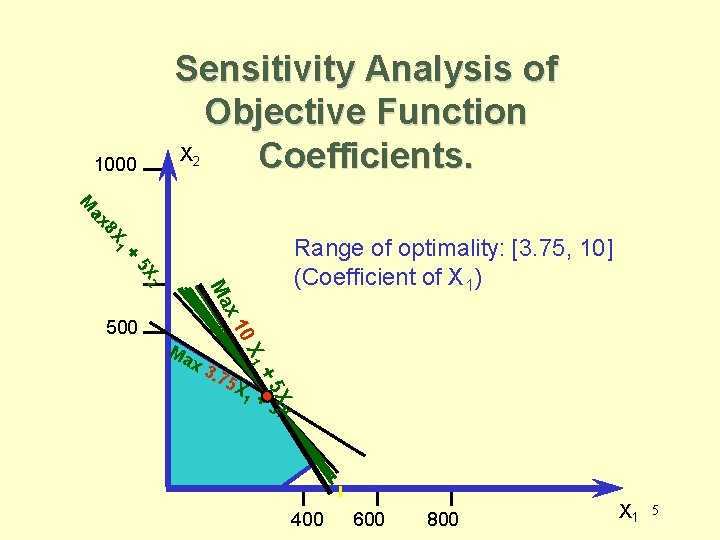
Sensitivity Analysis of Objective Function Coefficients. • Range of Optimality – The optimal solution will remain unchanged as long as • An objective function coefficient lies within its range of optimality • There are no changes in any other input parameters. – The value of the objective function will change 3

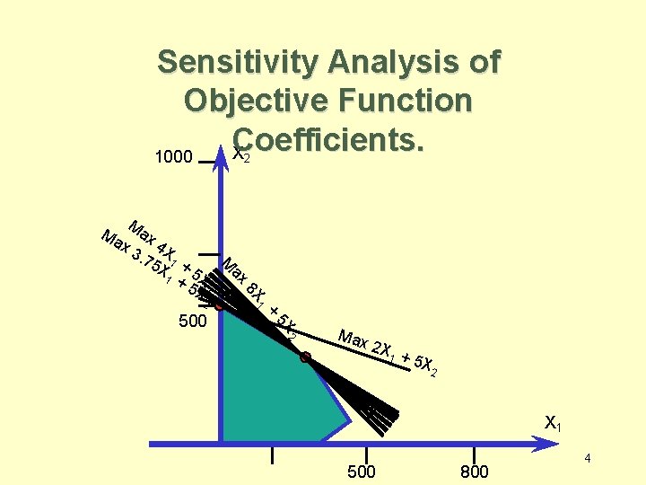
Sensitivity Analysis of Objective Function Coefficients. X 1000 2 M 8 X 1 + 5 X 500 ax 2 M ax x 3 4 X. 75 1 + X 5 X 2 Max 2 X 1 + 5 X 2 X 1 500 800 4

Sensitivity Analysis of Objective Function X Coefficients. 1000 2 8 X ax M 1 Range of optimality: [3. 75, 10] (Coefficient of X 1) + 5 X 1 +5 X 2 5 X +5 3. 7 1 Ma x 0 X x 1 Ma 2 500 X 2 400 600 800 X 1 5

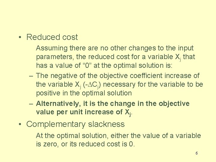
• Reduced cost Assuming there are no other changes to the input parameters, the reduced cost for a variable Xj that has a value of “ 0” at the optimal solution is: – The negative of the objective coefficient increase of the variable Xj (-DCj) necessary for the variable to be positive in the optimal solution – Alternatively, it is the change in the objective value per unit increase of Xj. • Complementary slackness At the optimal solution, either the value of a variable is zero, or its reduced cost is 0. 6

Sensitivity Analysis of Right-Hand Side Values • In sensitivity analysis of right-hand sides of constraints we are interested in the following questions: – Keeping all other factors the same, how much would the optimal value of the objective function (for example, the profit) change if the right-hand side of a constraint changed by one unit? – For how many additional or fewer units will this per unit change be valid? 7

Sensitivity Analysis of Right-Hand Side Values • Any change to the right hand side of a binding constraint will change the optimal solution. • Any change to the right-hand side of a non-binding constraint that is less than its slack or surplus, will cause no change in the optimal solution. 8

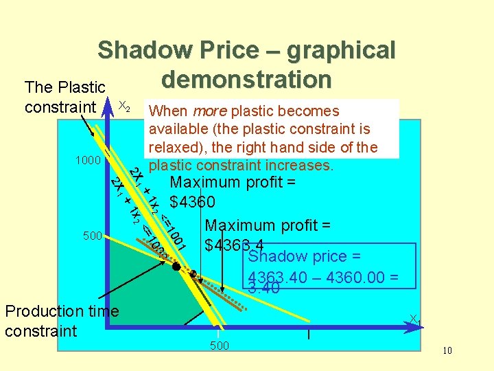
Shadow Prices • Assuming there are no other changes to the input parameters, the change to the objective function value per unit increase to a right hand side of a constraint is called the “Shadow Price” 9

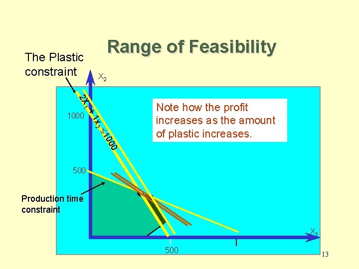
Shadow Price – graphical demonstration The Plastic constraint X 2 1000 Maximum profit = $4363. 4 Shadow price = 4363. 40 – 4360. 00 = 3. 40 01 10 <= 00 x 2 10 +1 <= x 2 +1 Production time constraint 2 X 1 500 When more plastic becomes available (the plastic constraint is relaxed), the right hand side of the plastic constraint increases. X 1 500 10

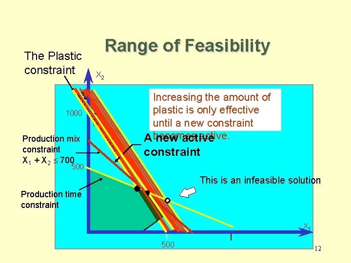
Range of Feasibility • Assuming there are no other changes to the input parameters, the range of feasibility is – The range of values for a right hand side of a constraint, in which the shadow prices for the constraints remain unchanged. – In the range of feasibility the objective function value changes as follows: Change in objective value = [Shadow price][Change in the right hand side value] 11

Range of Feasibility The Plastic constraint X 2 2 X 1 +1 1000 x 2 00 10 <= Production mix constraint X 1 + X 2 £ 700 Increasing the amount of plastic is only effective until a new constraint active. A becomes new active constraint 500 This is an infeasible solution Production time constraint X 1 500 12

Range of Feasibility The Plastic constraint X 2 2 X 1 +1 1000 x 2 0 00 £ 1 Note how the profit increases as the amount of plastic increases. 500 Production time constraint X 1 500 13

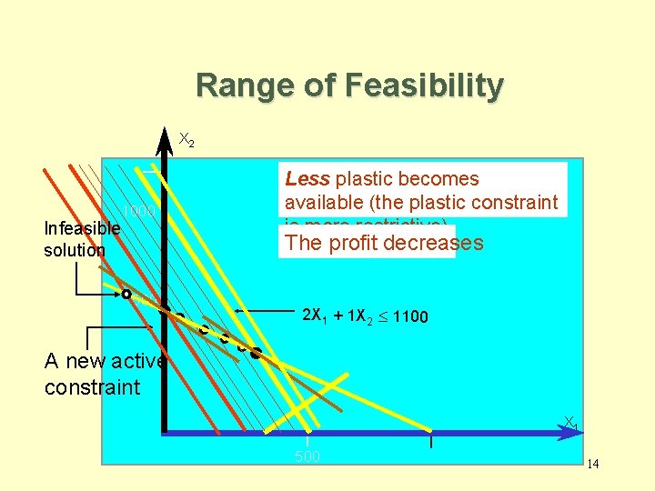
Range of Feasibility X 2 1000 Infeasible solution Less plastic becomes available (the plastic constraint is more restrictive). The profit decreases 500 2 X 1 + 1 X 2 £ 1100 A new active constraint X 1 500 14

Other Post - Optimality Changes • Addition of a constraint. • Deletion of a constraint. • Addition of a variable. • Deletion of a variable. • Changes in the left - hand side coefficients. 15

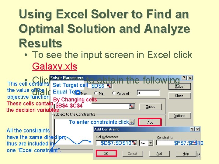
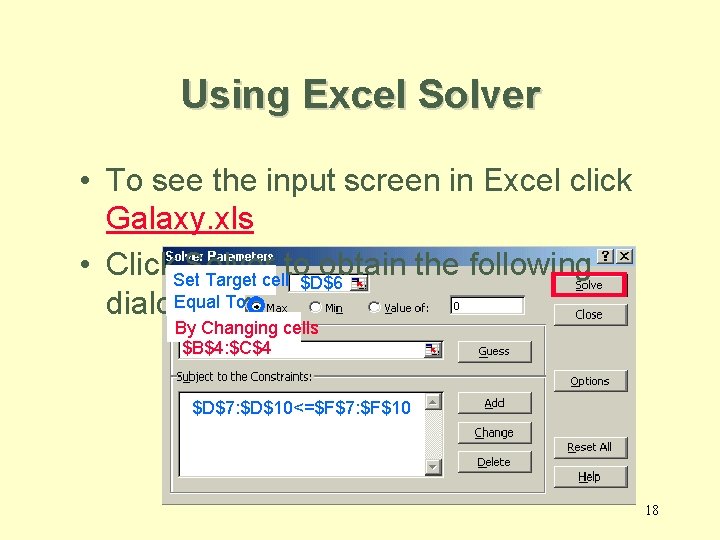
Using Excel Solver to Find an Optimal Solution and Analyze Results • To see the input screen in Excel click Galaxy. xls • contains Click. Set. Solver to obtain the following This cell Target cell $D$6 the value of the Equal To: dialog box. objective function By Changing cells These cells contain $B$4: $C$4 the decision variables To enter constraints click… All the constraints have the same direction, thus are included in one “Excel constraint”. $D$7: $D$10 $F$7: $F$10 16

Using Excel Solver • To see the input screen in Excel click Galaxy. xls • contains Click. Set. Solver to obtain the following This cell Target cell $D$6 the value of the Equal To: dialog box. objective function By Changing cells These cells contain $B$4: $C$4 the decision variables Click on ‘Options’ and check ‘Linear Programming’ and ‘Non-negative’. $D$7: $D$10<=$F$7: $F$10 17

Using Excel Solver • To see the input screen in Excel click Galaxy. xls • Click. Set. Solver to obtain the following Target cell $D$6 Equal To: dialog box. By Changing cells $B$4: $C$4 $D$7: $D$10<=$F$7: $F$10 18

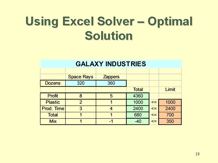
Using Excel Solver – Optimal Solution 19

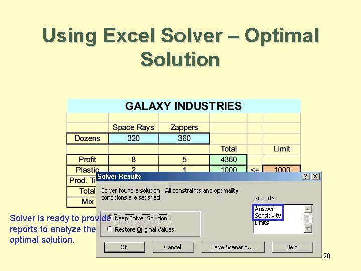
Using Excel Solver – Optimal Solution Solver is ready to provide reports to analyze the optimal solution. 20

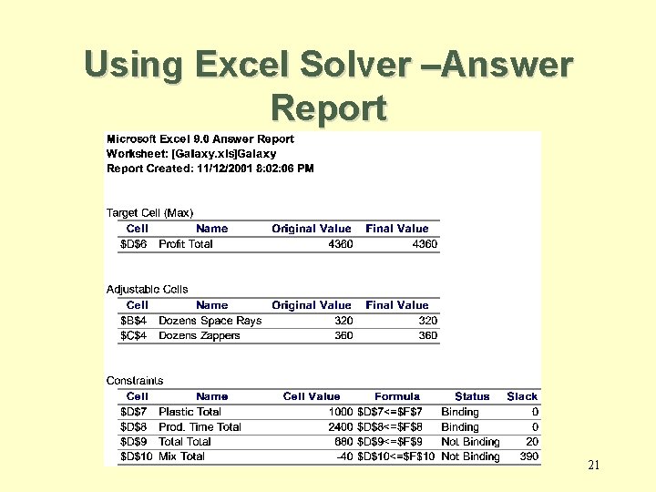
Using Excel Solver –Answer Report 21

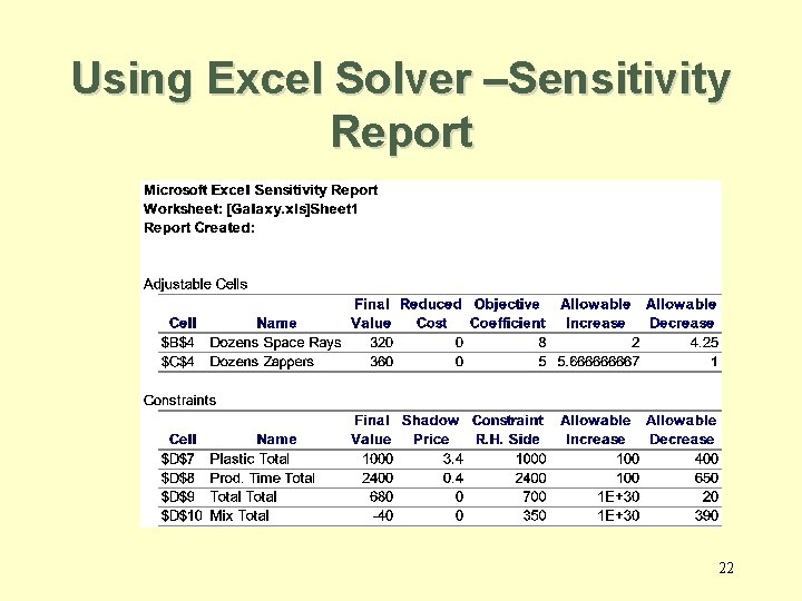
Using Excel Solver –Sensitivity Report 22

Another Example: Cost Minimization Diet Problem • Mix two sea ration products: Texfoods, Calration. • Minimize the total cost of the mix. • Meet the minimum requirements of Vitamin A, Vitamin D, and Iron. 23

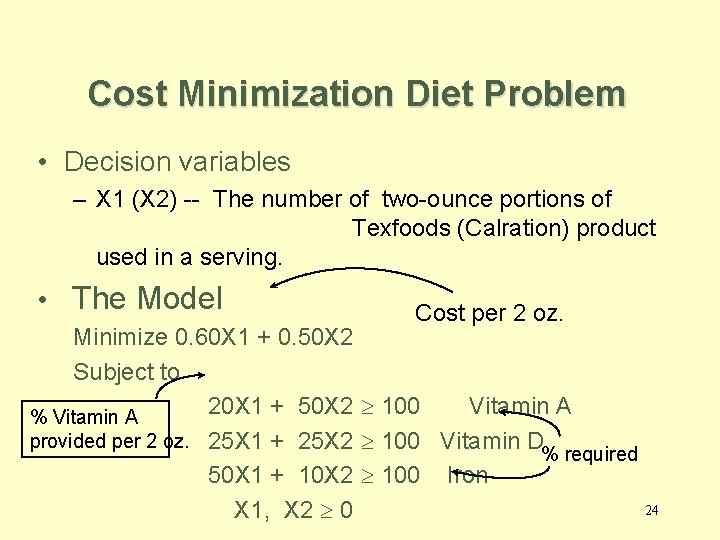
Cost Minimization Diet Problem • Decision variables – X 1 (X 2) -- The number of two-ounce portions of Texfoods (Calration) product used in a serving. • The Model Cost per 2 oz. Minimize 0. 60 X 1 + 0. 50 X 2 Subject to 20 X 1 + 50 X 2 ³ 100 Vitamin A % Vitamin A provided per 2 oz. 25 X 1 + 25 X 2 ³ 100 Vitamin D % required 50 X 1 + 10 X 2 ³ 100 Iron 24 X 1, X 2 ³ 0

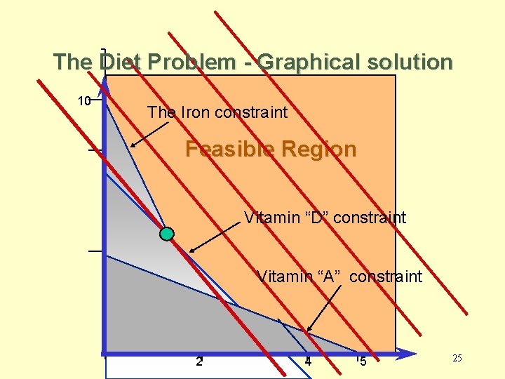
The Diet Problem - Graphical solution 10 The Iron constraint Feasible Region Vitamin “D” constraint Vitamin “A” constraint 2 4 5 25

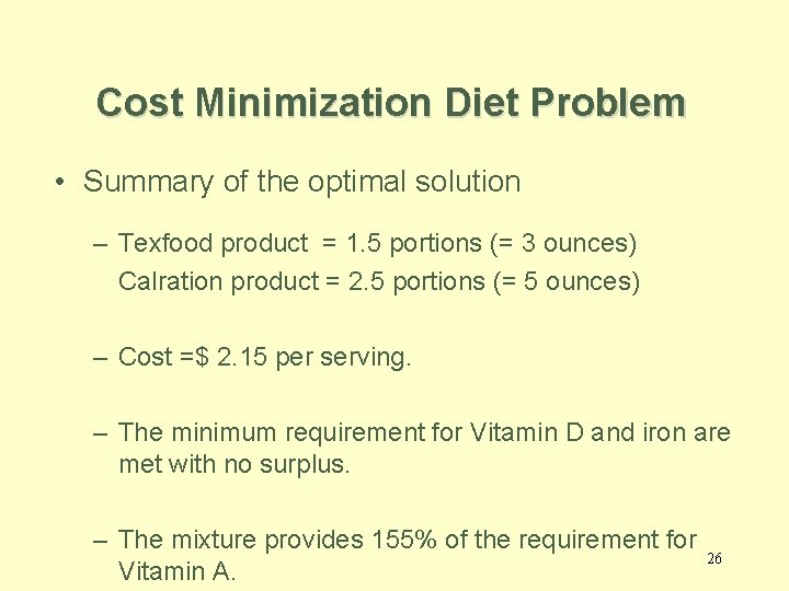
Cost Minimization Diet Problem • Summary of the optimal solution – Texfood product = 1. 5 portions (= 3 ounces) Calration product = 2. 5 portions (= 5 ounces) – Cost =$ 2. 15 per serving. – The minimum requirement for Vitamin D and iron are met with no surplus. – The mixture provides 155% of the requirement for Vitamin A. 26