The Receiver Operating Characteristic ROC Curve EPP 245298
- Slides: 9

The Receiver Operating Characteristic (ROC) Curve EPP 245/298 Statistical Analysis of Laboratory Data 1

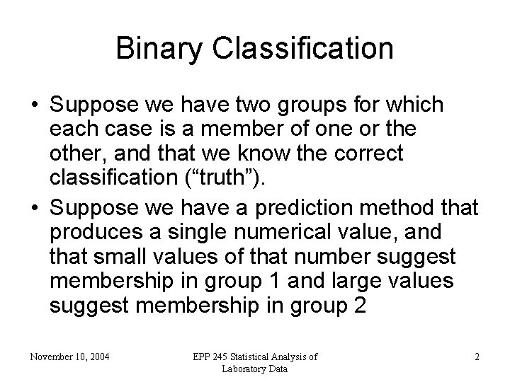
Binary Classification • Suppose we have two groups for which each case is a member of one or the other, and that we know the correct classification (“truth”). • Suppose we have a prediction method that produces a single numerical value, and that small values of that number suggest membership in group 1 and large values suggest membership in group 2 November 10, 2004 EPP 245 Statistical Analysis of Laboratory Data 2

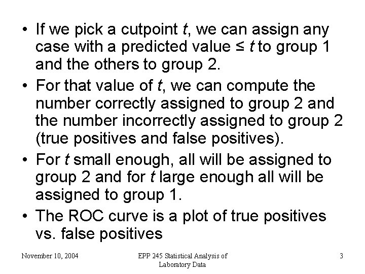
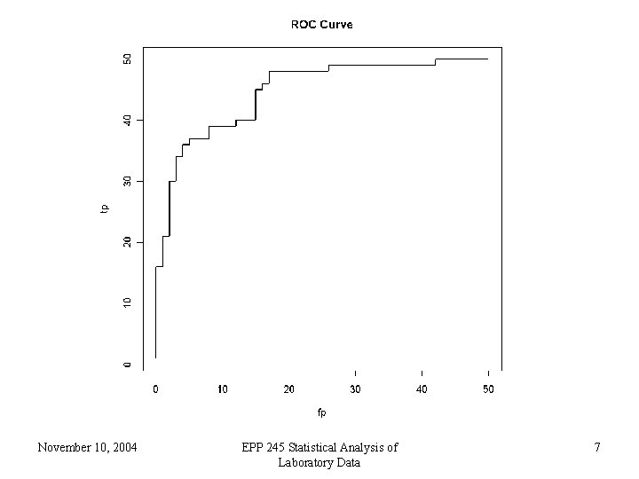
• If we pick a cutpoint t, we can assign any case with a predicted value ≤ t to group 1 and the others to group 2. • For that value of t, we can compute the number correctly assigned to group 2 and the number incorrectly assigned to group 2 (true positives and false positives). • For t small enough, all will be assigned to group 2 and for t large enough all will be assigned to group 1. • The ROC curve is a plot of true positives vs. false positives November 10, 2004 EPP 245 Statistical Analysis of Laboratory Data 3

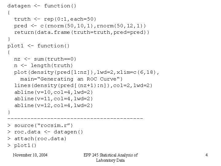
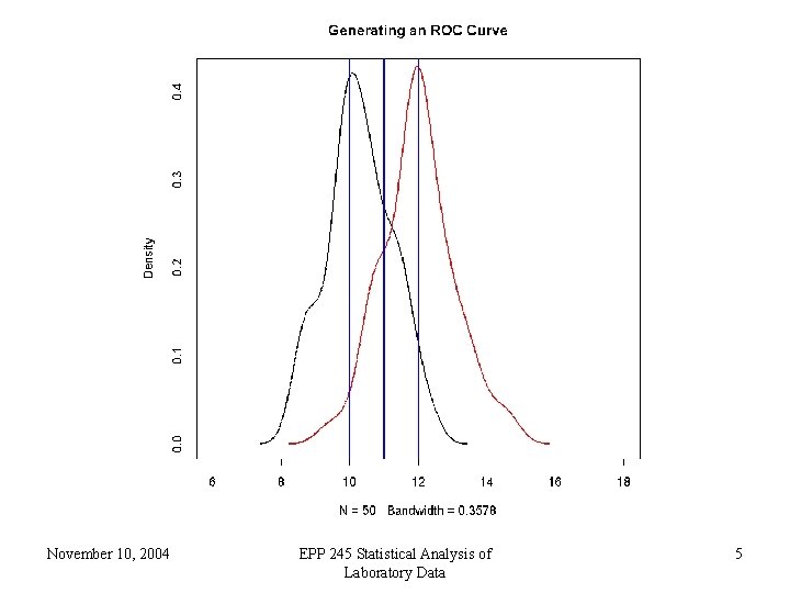
datagen <- function() { truth <- rep(0: 1, each=50) pred <- c(rnorm(50, 1), rnorm(50, 12, 1)) return(data. frame(truth=truth, pred=pred)) } plot 1 <- function() { nz <- sum(truth==0) n <- length(truth) plot(density(pred[1: nz]), lwd=2, xlim=c(6, 18), main="Generating an ROC Curve") lines(density(pred[(nz+1): n]), col=2, lwd=2) abline(v=10, col=4, lwd=2) abline(v=11, col=4, lwd=2) abline(v=12, col=4, lwd=2) } --------------------> source(“rocsim. r”) > roc. data <- datagen() > attach(roc. data) > plot 1() November 10, 2004 EPP 245 Statistical Analysis of Laboratory Data 4

November 10, 2004 EPP 245 Statistical Analysis of Laboratory Data 5

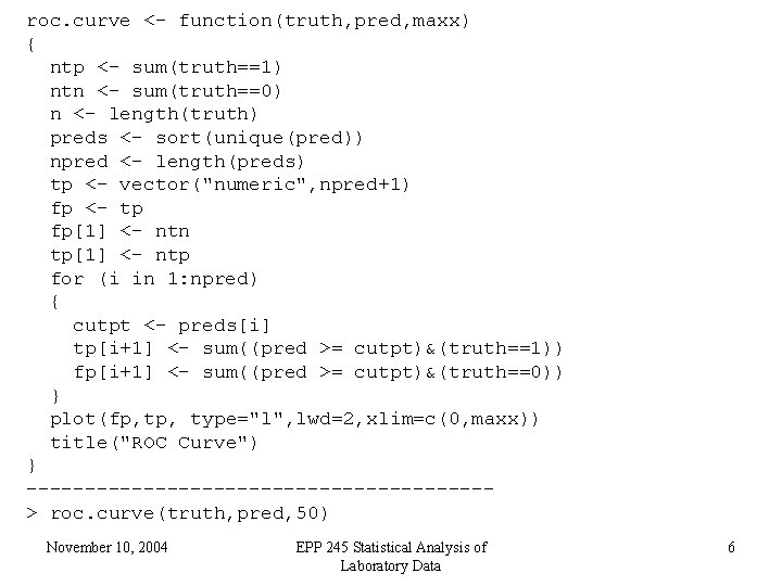
roc. curve <- function(truth, pred, maxx) { ntp <- sum(truth==1) ntn <- sum(truth==0) n <- length(truth) preds <- sort(unique(pred)) npred <- length(preds) tp <- vector("numeric", npred+1) fp <- tp fp[1] <- ntn tp[1] <- ntp for (i in 1: npred) { cutpt <- preds[i] tp[i+1] <- sum((pred >= cutpt)&(truth==1)) fp[i+1] <- sum((pred >= cutpt)&(truth==0)) } plot(fp, type="l", lwd=2, xlim=c(0, maxx)) title("ROC Curve") } --------------------> roc. curve(truth, pred, 50) November 10, 2004 EPP 245 Statistical Analysis of Laboratory Data 6

November 10, 2004 EPP 245 Statistical Analysis of Laboratory Data 7

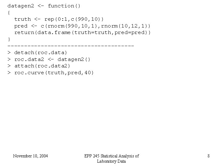
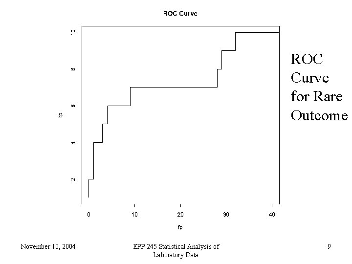
datagen 2 <- function() { truth <- rep(0: 1, c(990, 10)) pred <- c(rnorm(990, 1), rnorm(10, 12, 1)) return(data. frame(truth=truth, pred=pred)) } -------------------> detach(roc. data) > roc. data 2 <- datagen 2() > attach(roc. data 2) > roc. curve(truth, pred, 40) November 10, 2004 EPP 245 Statistical Analysis of Laboratory Data 8

ROC Curve for Rare Outcome November 10, 2004 EPP 245 Statistical Analysis of Laboratory Data 9