The Principle of Automatic Control LecturersProf Jiang Bin

The Principle of Automatic Control 自动控制原理 Lecturers:Prof. Jiang Bin Dr. Lu Ningyun College of Automation Engineering NUAA,2008. Autumn 1

NUAA-The Principle of Automatic Control Chapter 4 Root Locus Analysis 根轨迹分析 2

The Principle of Automatic Control 2008 Chapter 4 Root locus analysis • • • 4 -1 Introduction 4 -2 Root-locus equation 4 -3 Rules to draw regular root loci 4 -4 Generalized root loci 4 -5 Analysis of control system by RL method • 4 -6 Control system design by the rootlocus method 3

The Principle of Automatic Control 2008 Introduction Stability and the characteristics of transient response of closed-loop systems Locations of the closed-loop poles Problems to solve characteristic equation : 1. Difficult for a system of third or higher order. 2. Tedious for varying parameters. 4
 - K")
The Principle of Automatic Control 2008 Varying the loop gain K R(s) - K G (s) H(s) C(s) The open loop gain K is an important parameter that can affect the performance of a system • In many systems, simple gain adjustment may move the closed-loop poles to desired locations. • Then the design problem may become the selection of an appropriate gain value. • It is important to know how the closed-loop poles move in the s plane as the loop gain K is varied. 5

The Principle of Automatic Control 2008 Root locus method A simple method for finding the roots of the characteristic equation has been developed by W. R. Evans. This method is called root locus method. ØGraphical Analysis of Control System, AIEE Trans. Part II, 67(1948), pp. 547 -551. Ø Control System Synthesis by Root Locus Method, AIEE Trans. Part II, 69(1950), pp. 66 -69 6

The Principle of Automatic Control 2008 4 -2 Root-locus equation 8 8

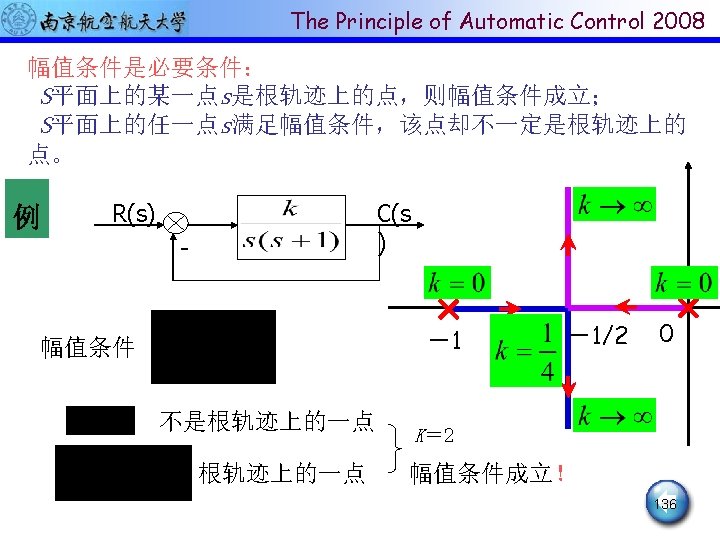
The Principle of Automatic Control 2008 Start from an example Consider a second-order system shown as follows: R(s ) - Y(s ) Closed-loop TF: Characteristic equation (CE): Roots of CE: The roots of CE change as the value of k changes. When k changes from 0 to ∞, how will the locus of the roots of CE move? 9 9

The Principle of Automatic Control 2008 k= 0 As the value of k increases, -1 the two negative real roots move closer to each other. -1/2 0 A pair of complex-conjugate roots leave the negative real-axis and move upwards and downwards following the line s=-1/2. On the s plane, using arrows to denote the direction of characteristic roots move when k increases, by numerical value to denote the gain at the poles. 10 10

The Principle of Automatic Control 2008 By Root loci, we can analyze the system behaviors (1)Stability: when Root loci are on the left half plane, then the system is definitely stable for all k>0. (2)Steady-state performance: there ’s an open-loop pole at s=0, so the system is a type I system. The steady-state error is 0 under step input signal v 0/Kv under ramp signal v 0 t ∞ under parabolic signal. 11 11
Transient performance: there’s a close relationship between root")
The Principle of Automatic Control 2008 (3)Transient performance: there’s a close relationship between root loci and system behavior on the real-axis: k<0. 25 underdamped; k=0. 25 critically damped k>0. 25 underdamped. However, it’s difficult to draw root loci directly by closed-loop characteristic roots-solving method. The idea of root loci : by loop transfer function, draw closed-loop root loci directly. 12
H(s) and")
The Principle of Automatic Control 2008 Relationship between zeros and poles of G(s)H(s) and closed-loop ones R(S) - G(s) Y(s) H(s) Forward path TF: Closed-loop TF: Feedback path TF: 13 13
 and H(s) into zero-pole-gain (zpk) form:")
The Principle of Automatic Control 2008 Write G(s) and H(s) into zero-pole-gain (zpk) form: RL gain of forward path RL gain of feedback path Zeros of forward path TF Poles of forward path TF Zeros of feedback path TF Poles of feedback path TF 14

The Principle of Automatic Control 2008 1. The closed-loop zeros = feed forward path zeros + feedback path poles. 2. The closed-loop poles are related to poles and zeros of G(s)H(s) and loop gain K. 3. The closed-loop root loci gain = the feed forward path root loci gain. 15

The Principle of Automatic Control 2008 Root-locus equation To draw Closed-loop root locus is to solve the CE That is RL equation Suppose that G(s)H(s) has m zeros (Zi) and n poles( Pi), the above equation can be re-written as K* varies from 0 to ∞ 16 16
H(s) is function of a")
The Principle of Automatic Control 2008 RL equation: Since G(s)H(s) is function of a complex variable s, the root locus equation can be described by the following two equations: Magnitude equation (ME) Magnitude equation is related not only to zeros and poles of G(s)H(s), but also to RL gain ; Angle equation (AE) Angel equation is only related to zero and poles of G(s)H(s). Use AE to draw root loci and use ME to determine the value of K on root loci. 17 17
H(s)(×) Zeros of G(s)H(s)(〇)")
Example 1 The Principle of Automatic Control 2008 Poles of G(s)H(s)(×) Zeros of G(s)H(s)(〇) For a point s 1 on the root loci, use AE Use ME Angel is in the direction of anticlockwise 18 18

Example 2 The Principle of Automatic Control 2008 Unity-feedback transfer function: One pole of G(s)H(s): No zero. Test a point s 1 on the negative real-axis All the points on the negative real-axis are on RL. Test a point outside the negative real-axis s 2=-1 -j 19 All the points outside the negative real-axis are not on RL. 19

The Principle of Automatic Control 2008 Probe by each point: 1. Find all the points that satisfy the Angle Equation on the s-plane, and then link all these points into a smooth curve, thus we have the system root locus when k* changes from 0 to ∞; 2. As for the given k, find the points that satisfy the Magnitude Equation on the root locus, then these points are required closed-loop poles. However, it’s unrealistic to apply such “probe by each point” method. W. R. Evans (1948) proposed a set of root loci drawing rules which simplify the our drawing work. 20

The Principle of Automatic Control 2008 4 -3 Rules to draw regular root loci (suppose the varying parameter is open-loop gain K ) 21 21

The Principle of Automatic Control 2008 Properties of Root Loci 1 and points of Root Loci 2 Number of Branches on the RL 3 Symmetry of the RL 4 Root Loci on the real-axis 5 Asymptotes of the RL 6 Breakaway points on the RL 7 Departure angle and arrival angle of RL 8 Intersection of the RL with the imaginary axis 9 The sum of the roots and the product of the roots of the closed-loop characteristic equation 22

The Principle of Automatic Control 2008 1 and points Root loci originate on the poles of G(s)H(s) (for K=0) and terminates on the zeros of G(s)H(s) (as K=∞). RL Equation: Magnitude Equation: Root loci start from poles of G(s)H(s) Root loci end at zeros of G(s)H(s). 23 23

The Principle of Automatic Control 2008 2 Number of branches on the RL nth-order system, RL have n starting points and RL have n branches RL Equation: The order of the characteristic equation is n as K varies from 0 to ∞ , n roots change n root loci. For a real physical system, the number of poles of G(s)H(s) are more than zeros,i. e. n > m. n root loci end at open-loop zeros(finite zeros); m root loci end at open-loop zeros(finite zeros); (n-m)root loci end at (n-m) infinite zeros. 24 24

The Principle of Automatic Control 2008 3 Symmetry of the RL The RL are symmetrical with respect to the real axis of the The s-plane. roots of characteristic equation are real or complex -conjugate. Therefore, we only need to draw the RL on the up half s-plane and on the real-axis, the rest can be obtained by plotting its mirror image. 25 25

The Principle of Automatic Control 2008 4 RL on the Real Axis On a given section of the real axis, RL for k>0 are found in the section only if the total number of poles and zeros of G(s)H(s) to the right of the section is odd. zero:z 1 poles:p 1、p 2、p 3、p 4、p 5 Pick a test point s 1 on [p 2,p 3] ? The sum of angles provided by every pair of complex conjugate poles are 360°; The angle provided by all the poles and zeros on the right of s 1 is 180°; The angle provided by all the poles and zeros on the left of s 1 is 0°. 26 26

Example Consider the following loop transfer function The Principle of Automatic Control 2008 Determine its root loci on the real axis. Poles: jw Zeros: S-plane Repeated poles: -6 -5 -4 -3 -2 -1 0 On the right of [-2,-1] the number of real zeros and poles=3. On the right of [-6,-4], the number of real zeros and poles=7. 27 27

The Principle of Automatic Control 2008 5 Asymptotes of RL When n ≠ m, there will be 2|n-m| asymptotes that describe the behavior of the RL at |s|=∞. RL Equation: The angles between the asymptotes and the real axis are(i= 0,1,2,… , n-m-1) : The asymptotes intersect the real axis at: 28 28

Example Consider the following loop transfer function The Principle of Automatic Control 2008 Determine the asymptotes of its root loci. 3 poles: 0、-1、-5 n-m = 3 -1 = 2 1 zero:-4 The asymptotes intersect the real axis at The angles between the asymptotes and the real axis are 29 29

Example Consider the following loop transfer function The Principle of Automatic Control 2008 Determine the asymptotes of its root loci. 4 poles: 0、-1+j、-1 -j、-4 n-m=4 -1=3 1 zero:-1 The asymptotes intersect the real axis at The angles between the asymptotes and the real axis are 30 30

of Automatic Control 2008 6 Breakaway points. The on. Principle the RL Breakaway points on the RL correspond to multi-order roots of the RL equation. The breakaway points on the RL are determined by finding the roots of d. K/ds=0 or d. G(s)H(s)=0. 31 31

Method-1 The Principle ofof Automatic Control 2008 The breakaway point b is the solution Proof: Suppose the multi-order root is s 1,then we have 32 32
 divided by (1) yields Thus Or Solutions")
The Principle of Automatic Control 2008 (2) divided by (1) yields Thus Or Solutions 1 is the breakaway point b 33
H(s) are shown. Control in the 2008 The")
Example -3 The poles and zeros G(s)H(s) are shown. Control in the 2008 The of Principle of Automatic following figure, determine its root loci. jω Rule 1、2、3 -2 -1 0 σ RL have three branches,starting from poles 0、-2、-3,ending at on finite zero -1 and two infinite zeros. The RL are symmetrical with respect to the real axis. Ruel 4 The intersections [-1, 0] and[-3, -2] on the real axis are RL. Rule 5 The RL have two asymptotes(n-m= 2) Rule 6 The RL have breakaway points on the real axis (within[-3, -2]) 34 34

The breakaway point b is the solution of of Automatic Control The Principle 2008 Method-2 Proof: Suppose s moves from p 2 to p 1, if we increase K from zero,K reaches its maximum when s reaches b. Then K decreases and reaches zero at p 1. K corresponding to the breakaway point has the maximum value. Thus 35 35

Example The Principle of Automatic Control 2008 jω -4 -2 Rule 1、2、3、4 n=4, m=0 j 4 0 σ the RL are symmetrical with respect to the real axis; the RL have four branches which start from poles 0, -4 and -2±j 4 ; the RL end at infinite zeros; the intersection [-4, 0] on the realaxis is RL Rule 5 The RL have four asymptotes. -j 4 36 36

Example The Principle of Automatic Control 2008 jω -4 -2 Rule 6 the breakaway point of the RL j 4 0 σ -j 4 37 37

The Principle of of Automatic 2008 7 Angles of departure and angles arrival. Control of the RL The angle of departure or arrival of a root locus at a pole or zero, respectively, of G(s)H(s) denotes the angle of the tangent to the locus near the point. 38 38

Angle of Departure: The Principle of Automatic Control 2008 Pick up a point s 1 that is close to p 1 Applying Angle Equation (AE) s 1 p 1 angle of departure θp 1 39 39

Angle of Arrival: The Principle of Automatic Control 2008 40 40

Example The Principle of Automatic Control 2008 Consider the following loop transfer function Determine its RL when K varies from 0 to ∞. 3 poles P 1, 2=-1(repeated poles) P 3=1; 1 zero Z 1=0,n-m=2。 3 branches ,2 asymptotes j -1 -0. 5 1 Angle of departure: 41 41

of Automatic Control 2008 8 Intersection of The the. Principle RL with the Imaginary Axis Intersection of the RL with Im-axis ? The characteristic equation have roots on the Im-axis and the system is marginally stable. Method 1 Use Routh’s criterion to obtain the value of K when the system is marginally stable, the get ω from K. Method 2 42 42

Example Consider the following loop transfer function The Principle of Automatic Control 2008 Determine the intersection of the RL with Im-axis. Method 1 Closed-loop CE: Routh’s Tabulation: Marginally stable: K =6 Auxiliary equation: Intersection point: 43 43

Example Consider the following loop transfer function The Principle of Automatic Control 2008 Determine the intersection of the RL with Im-axis. Method 2 Closed-loop CE: →Closed-loop CE 44 44

The Principle of Automatic Control 2008 Summary of General Rules for Constructing Root Loci R(S) First, obtain the characteristic equation (CE) - G(s) Y(s) H(s) Then, rearrange the equation so that the parameters of interest appear as the multiplying factor in the form We sketch the Root Loci when K>0 varies from 0 to ∞. 45

The Principle of Automatic Control 2008 Step 1: Locate the poles and zeros of G(s)H(s) on the splane. The RL start from poles of G(s)H(s) and terminate at zeros (finite zeros or zeros at infinity) Step 2: Determine the RL on the real-axis. Choose a test point on the real-axis, if the total number of real poles and real zeros to the right of the test is odd, then the test point is on the RL. Step 3: Determine the asymptotes of RL. The angles between the asymptotes and the real axis are(i= 0,1,2,… , n-m-1) : The asymptotes intersect the real-axis at: 46

The Principle of Automatic Control 2008 Step 4: Determine the breakaway and break-in points. The breakaway and break-in points can be determined by finding the roots of Step 5: Determine the angle of departure (angle of arrival) of the RL from a complex pole (at a complex zero) Angle of departure from a complex pole pj= Angle of arrival at a complex zero zk= 47

The Principle of Automatic Control 2008 Step 6: Find the points where the RL may cross the imaginary-axis. Method 1 Use Routh’s criterion to obtain the value of K when the system is marginally stable, the get ω from K. Method 2 48

Example Consider a unity feedback with Control the open. The Principle system of Automatic 2008 loop transfer function as: Sketch RL of the closed-loop system when K varies from 0 to ∞. Solution. loop TF: Step 1: Locate the poles and zeros of G(s)H(s) on the splane. loop poles: p 1=0, p 2=-3, p 3, 4=-1±j, n=4; no loop zeros: m=0; 49 49

The Principle of Automatic Control 2008 Step 2: Determine the RL on the real-axis. The section [0, -3] of the real axis are RL. 1. 5 Step 3: Determine the asymptotes of RL The angles between the asymptotes and the real axis are(i= 0, 1,2,… , n-m-1) : The asymptotes intersect the real-axis at: 1 0. 5 -3 -2. 5 -2 -1. 5 -1 0 -0. 5 50 50

The Principle of Automatic Control 2008 Step 4: Determine the breakaway and break-in points. 1. 5 1 0. 5 -3 -2. 5 -2 -1. 5 -1 0 -0. 5 51 51

Step 5: Determine the angle The of Principle of Automatic Control 2008 departure (angle of arrival) of the RL from a complex pole (at a complex zero) 1. 5 1 0. 5 -3 -2. 5 -2 -1. 5 -1 0 -0. 5 Using measurement to estimate 52 52

Step 6: Find the points The Principle of Automatic Control 2008 where the RL may cross the imaginary-axis. The characteristic equation: 1. 5 1 Substituting S=jw into the above equation yields: 0. 5 -3 -2. 5 -2 -1. 5 -1 0 -0. 5 53 53

The Principle of Automatic Control 2008 The complete RL: 1. 5 1 0. 5 -3 -2. 5 -2 -1. 5 -1 -0. 5 0 54 54

The Principle of Automatic Control 2008 To draw RL using MATLAB 特征方程: >>n=1; d=[1 3 2 0]; >>sys=tf(n, d); >>rlocus(sys) 注意: K*一变,一组根全变 一组根对应同一个K* K*一停,一组根都停 55

The Principle of Automatic Control 2008 56

The Principle of Automatic Control 2008 Determination of closed-loop poles 闭环极点的确定 Every point on the RL represents a closed-loop pole corresponding to a certain value of K which can be determined according to the Magnitude Equation。 Magnitude Equation : 57

unity feedback system whose Thea Principle of Automatic Control 2008 Example Given the RL of open-loop transfer function is: Determine the closed-loop poles when K =4. 1. 5 jw=-1. 1 1 0. 5 d=-2. 3 -3 -2. 5 -2 -1. 5 -1 -0. 5 0 58

Thepole Principle of Automatic Control 2008 Determine the closed-loop Magnitude Equation : according to ME: 4 poles,no zero At the breakaway point d=-2. 3, its corresponding K=4. 3 K increases from 0 to 4. 3 So there are exist the two real closed-loop poles locating at two sides of the breakaway point corresponding to K=4 Pick two points within [-3, -2. 3] and [-2. 3, 0] , using trial-and-error(试探) to find the closed-loop poles on the real-axis. 59
 to get")
The Principle of Automatic Control 2008 Closed-loop CE: Using the ‘Synthetic Division’(长除法) to get 60

The Principle of Automatic Control 2008 也可由根之和, 根之积与方程式系数的关系解出 So when K=4, the closed-loop transfer function is 61
 j j j 0 0 0")
The Principle of Automatic Control 2008 根轨迹示例 1(demos) j j j 0 0 0 j j 0 0 62

The Principle of Automatic Control 2008 根轨迹示例2 j j 0 0 j j jj 0 j 0 0 63

The Principle of Automatic Control 2008 4 -4 Generalized Root Loci 广义根轨迹 64

The Principle of Automatic Control 2008 Introduction 以开环增益K为可变参数绘制的根轨迹为Regular RL--For negative feedback system. 以非开环增益K为可变参数绘制的根轨迹为 Generalized RL. 参量根轨迹(变化开环零点,变化开环极点) 零度根轨迹(正反馈系统, positive-feedback system) 如果引入equivalent open-loop transfer function 的概念, 则广义根轨迹的绘制方法与常规根轨迹完全 相同。 65

The Principle of Automatic Control 2008 RL for the case of varying open-loop zeros Example 1. Given a system’s structure diagram, where the parameter is speed feedback constant. Problem: Draw RL when varies from 0 to ∞. C(s) R(s) - 1+ s 66

The Principle of Automatic Control 2008 From the structure diagram, the open-loop transfer function is R(s) C(s) 1+ s The closed-loop transfer function is: 67

The Principle of Automatic Control 2008 The characteristic equation is: It can be re-written as Define The is the equivalent open-loop transfer function whose open-loop gain is just the parameter of the original system. 68
")
The Principle of Automatic Control 2008 The new system is shown as follows: R(s) C(s) - The closed-loop transfer function : Note: The same denominator, but different numerator, compared with the original system. 69

The Principle of Automatic Control 2008 For the new system : 2 poles, 1 zero , i. e. n=2, m=1 2 branches, one approaches to zero, the other approaches to inf There are RL on the real axis [-inf 0] jω 3 2 1 -4 -3 -2 σ -1 70
和原系统一致,但分子(零点)不一致。因此 该方法can only determine system closed-loop")
The Principle of Automatic Control 2008 等效开环传递函数方法的重要说明 通过等效开环传递函数绘制的根轨迹,等效系统闭环传函的 分母(极点)和原系统一致,但分子(零点)不一致。因此 该方法can only determine system closed-loop poles, we still need to determine the system closed-loop zeros to analyze system dynamic behavior. Analysis of the influence of variation of Kt on the system R(s) C(s) 1+ s When Kt varies from 0 to infinity, an zero is added to the loop function G(s)H(s) and the zero moves from the negative infinity to the origin of s-plane. 71
 When Kt is small, a pair of")
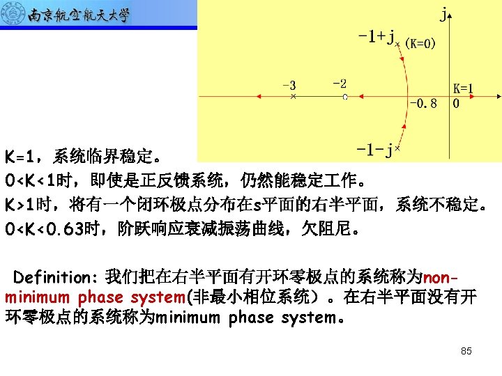
The Principle of Automatic Control 2008 R(s) When Kt is small, a pair of closed-loop complex-conjugate poles are close to the Im-axis, the overshoot of system step response is large and the oscillation is 1+ s jω strong. When Kt is small, the system velocity feedback signal is weak and underdamped. When Kt increases, the system damp is enhanced, the oscillation is weaken and the overshoot decreases, the system behavior is enhanced. The breakaway point: Kt= 0. 43,the -4 -3 -2 -1 system is critically damped. When Kt>0. 43, the two closed-loop poles are negative and real , the system is overdamped. Adding left-half plane zeros to open-loop transfer function generally has the effect of moving and bending the root loci toward the left-half s-plane. (4 -5节继续讲解) C(s) 3 2 1 σ 72

The Principle of Automatic Control 2008 RL for the case of varying open-loop poles Example 2: Consider a unity feedback system whose open-loop transfer function is where K and T are given constants, while the parameterτ is to be determined. Problem: Draw RL whenτvaries from 0 to infinity. 73
H(s)=0 The equivalent open loop")
The Principle of Automatic Control 2008 The characteristic equation: 1+G(s)H(s)=0 The equivalent open loop transfer function G 1(s): Solving Suppose that 4 KT>1, then two complex poles of G(S) are: 74

The Principle of Automatic Control 2008 2 poles, 3 zeros Z 1=Z 2=0, Z 3=-1/T So number of branches of the RL is equal to 3. According to rule 8, the interaction point with the imaginary axis is determined by 1+G 1(jw)=0, that is It follows that 75

The Principle of Automatic Control 2008 RL whenτvaries from 0 to infinity is shown as follows: the system is unstable. Note: Adding a pole to open-loop transfer function has The effect of pushing the RL toward the right-half plane (4 -5节继续讲解) 76
 R(S) + G(s) H(s) C(S) 称负反馈系统的根轨")
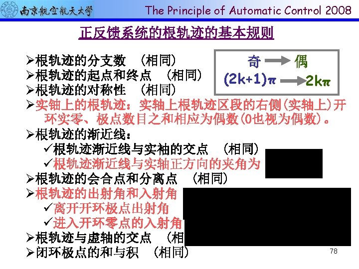
The Principle of Automatic Control 2008 Zero-degree RL(零度根轨迹) R(S) + G(s) H(s) C(S) 称负反馈系统的根轨 迹为 180°根轨迹。正 反馈的根轨迹称为 zero-degree RL(零 度根轨迹) The characteristic equation of positive feedback loop is 1 -G(s)H(s)=0, that is G(s)H(s)=1 Magnitude equation is Angle equation is 77
 C(s) + The open-loop")
The Principle of Automatic Control 2008 例 已知系统结构图,要求绘制K*由 0变化到inf的根轨迹 R(s) C(s) + The open-loop TF: (1) Plot the open-loop poles (n=3, P 1=-3, P 2=-1+j, P 3=-1 -j) and zero (m=1, Z 1=-2) 79

The Principle of Automatic Control 2008 -1+j -3 j 0 -2 -1 -j As K is increased from 0 to inf, the CL poles start at the OL poles and terminate at the OL zeros (same as in negative feedback system) (2)Determine the root loci on the real axis. Root loci exists on [-2, +∞)and (-∞, -3]. (实轴上从右向左数, 凡 偶数零极点左边的一段是根轨迹, 第一个零极点右边的实轴也 是根轨迹。) 80
")
The Principle of Automatic Control 2008 -1+j -3 -2 j 0 -1 -j (3) Determine the asymptotes of the root loci. n-m=2, two asymptotes Indicate that the asymptotes are on the real axis (4) Find the angle of departure of the root locus from a complex poles 81
 Determine the breakaway and break-in points -1+j")
The Principle of Automatic Control 2008 (5) Determine the breakaway and break-in points -1+j -3 j 0 -2 -1 -j 82
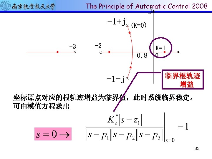

The Principle of Automatic Control 2008 开环传递函数 开环增益 84
 设 G(s)= 2+4 s+16)")
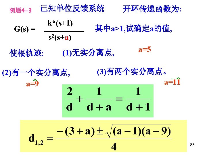
The Principle of Automatic Control 2008 例题 4 -1 k*(s+1) 设 G(s)= 2+4 s+16) s(s-1)(s θp 1= -54. 5 o 试绘制概略根轨迹。 σ = -2/3 -2+j 3. 46 j a j 1. 56 K*=23. 3 解: 给出如下计算参数 分离点:d 1,2= 0. 46, -2. 22 渐近线:σa= -2/3, o, 180 o-1 φa=d =± 60 2 -2. 22 0 起始角:± 54. 5 o 1 d 1=0. 46 与虚轴交点: -j 2. 56 k 1*=23. 3, s 1, 2=±j 1. 56 K*=35. 7 k 2*=35. 7, s 1, 2=±j 2. 56 86

j 例题 4 -2 s=0. 7 j The Principle of Automatic Control 2008 已知单位反馈系 统根轨迹如图所示 1 求闭环出现重根时 k 1=0. 332 -1 -2 0 d 2= -1. 37 Φ(s)的零极点表达式 1 d 1=0. 366 k 1=0. 0718 k 2=13. 9 2 求欠阻尼状态下单位斜坡输入时ess的范围 解: 1 Φ(s)= k 1=0. 0718 k 2= 0. 332 k 3= 13. 9 0. 067(s+1)(s+2) (s-0. 366)2 0. 933(s+1)(s+2) (s+1. 37)2 2 k= -2 k* ess=1/k -1. 5<ess<-0. 036 87
 = k*(s+1) 4 -3图 s 2(s+a)")
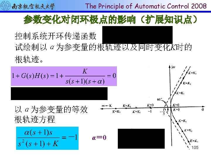
The Principle of Automatic Control 2008 例题 G(s) = k*(s+1) 4 -3图 s 2(s+a) j -5 a=9 a=11 j -1 0 -9 -1 -1 0 j j j -5 j 0 -9 -3 -1 0 -11 -4. 62 -2. 38 -1 89 例题 4 -3图 0
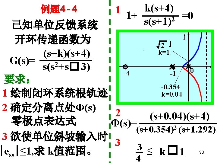

The Principle of Automatic Control 2008 On-class exercise Consider the unity-feedback control system with the following open-loop transfer function, a>0 Sketch the root loci. 91
 92")
The Principle of Automatic Control 2008 习题 (a>0) 92

The Principle of Automatic Control 2008 补充习题 93

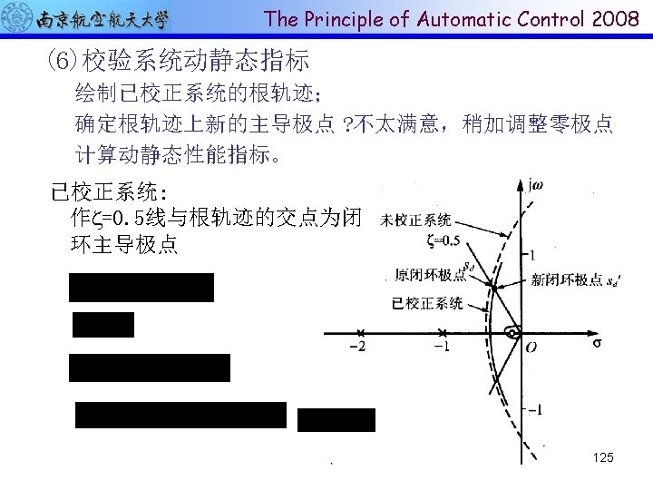
The Principle of Automatic Control 2008 4 -5 Analysis of control system the root -locus method ( 补充内容) 94
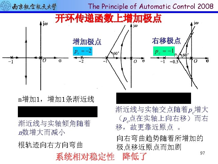
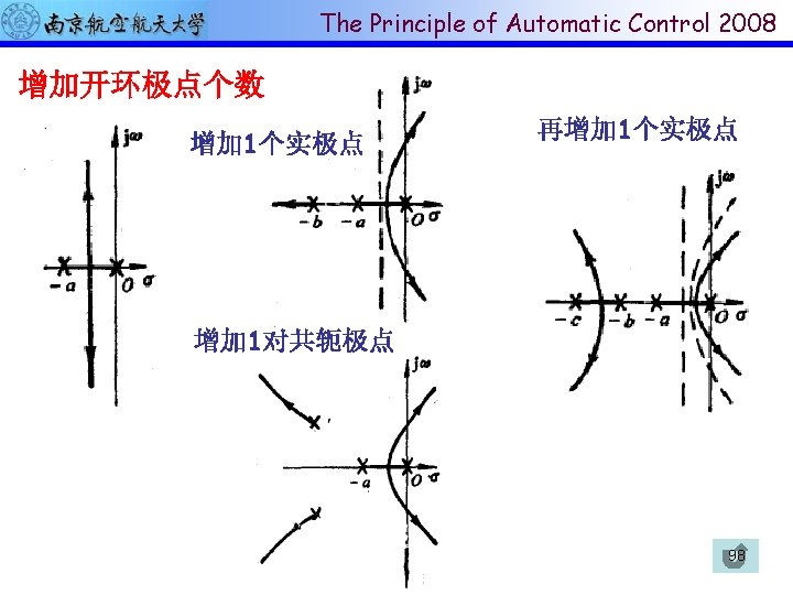
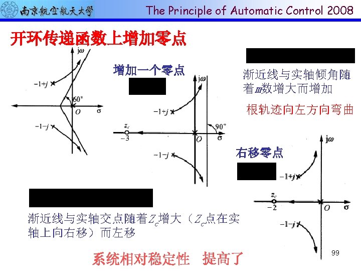

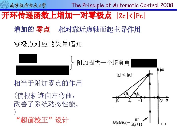
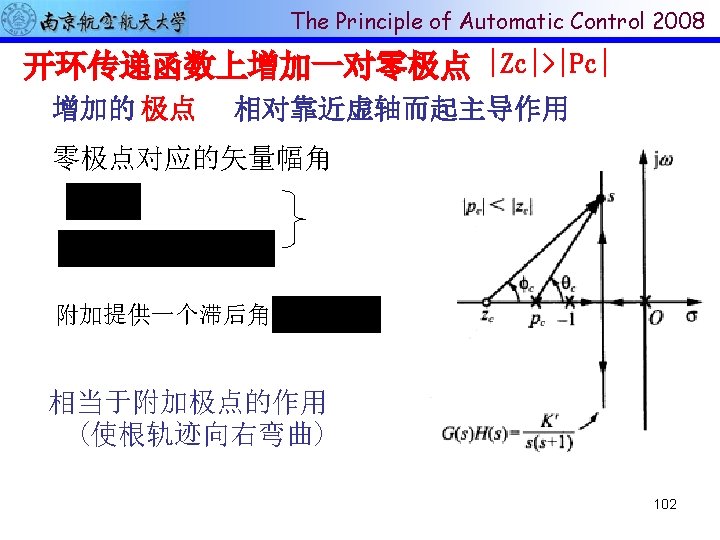
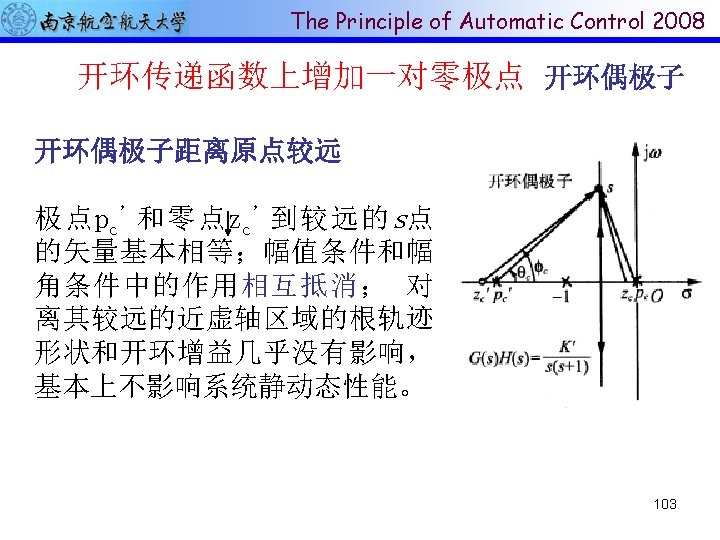
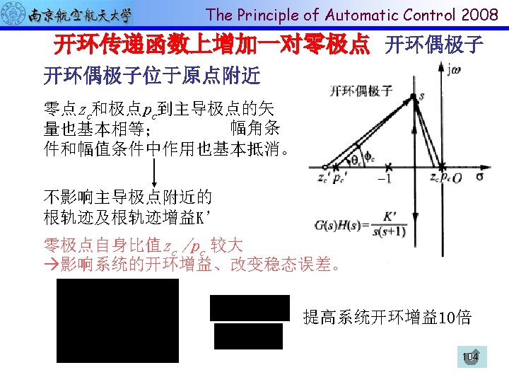
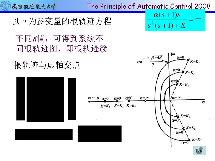
The Principle of Automatic Control 2008 增加开环零点个数 100

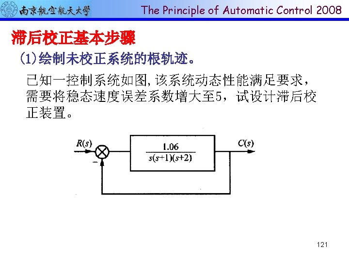
The Principle of Automatic Control 2008 4 -6 Control system design by RL method (补充内容) 110

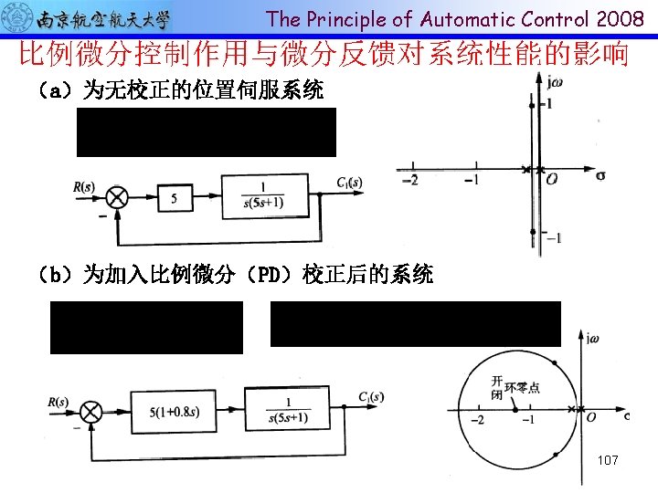
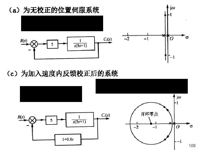
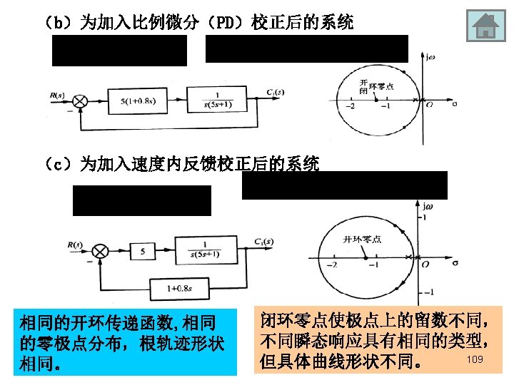
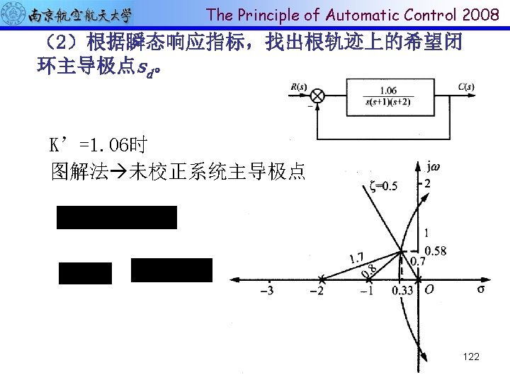
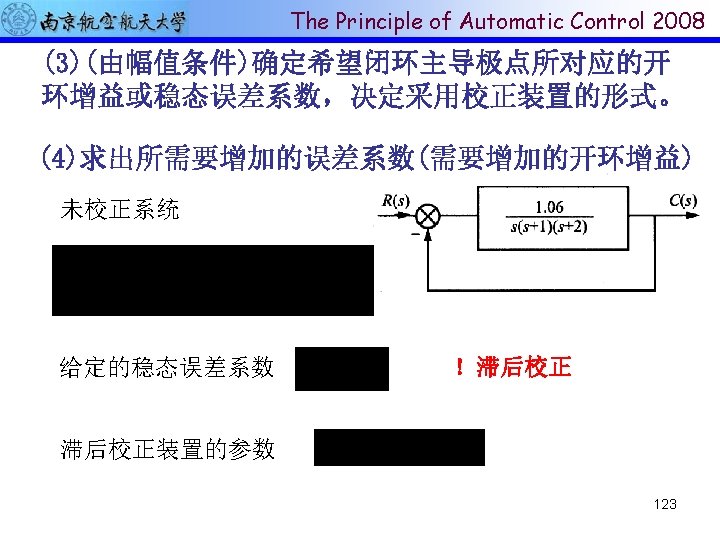
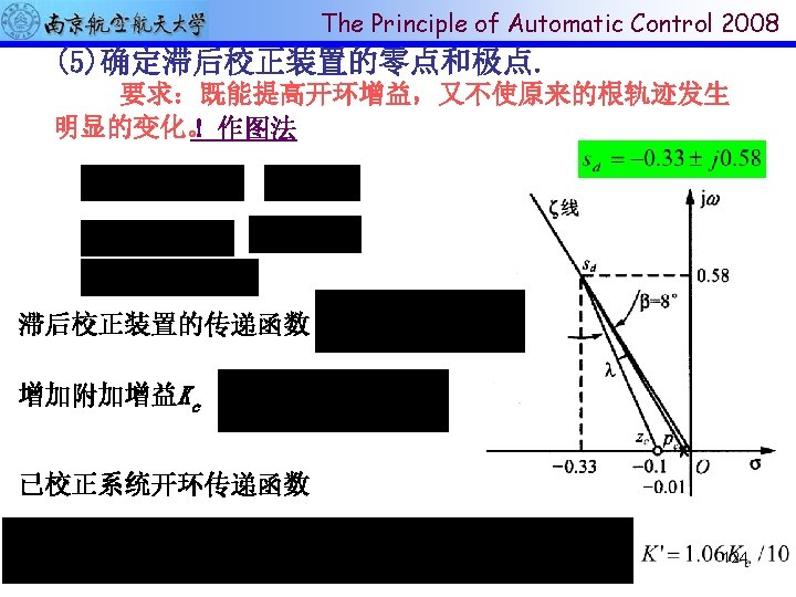
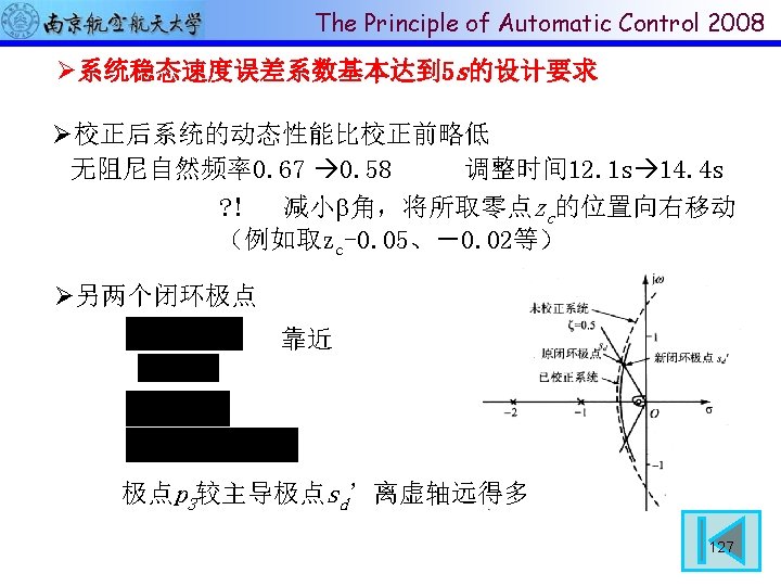
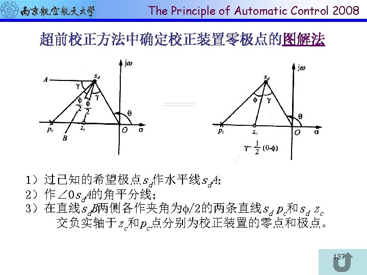
The Principle of Automatic Control 2008 Key Idea The design by the root-locus method is based on reshaping the toot locus of the system by adding poles and zeros to the systems open loop transfer function and forcing the root loci to pass through desired closed loop poles in s plane The characteristic of the root locus design is based on the assumption that the closed-loop system has a pair of dominant closed-loop poles. 111

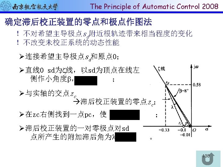
The Principle of Automatic Control 2008 System compensation Setting the gain is the first step in adjusting the system for satisfactory performance. – Improve steady state behavior but result in poor stability or instability Redesign the system to alter the overall behavior to achieve desired performance by modifying the structure or incorporating additional devices or components is called compensation(补偿),such devices is a compensator(补偿器) – Lead, Lag-lead, PID controller 112

End of Chapter 4 Thank you all! 139
- Slides: 139