The Power of Proc Nlmixed Introduction Proc Nlmixed

The Power of Proc Nlmixed

Introduction • Proc Nlmixed fits nonlinear mixed-effects models (NLMMs) – models in which the fixed and random effects have a nonlinear relationship • NLMMs are widespread in pharmacokinetics – ? genesis of procedure • Nlmixed was first available in Version 7 (experimental) and then in Version 8 (production)

Introduction (cont. ) • Nlmixed is similar to the Nlinmix and Glimmix macros but uses a different estimation method, and is much easier to use • Macros iteratively fit a set of GEEs, whereas Nlmixed directly maximizes an approximation of the likelihood, integrated over the random effects

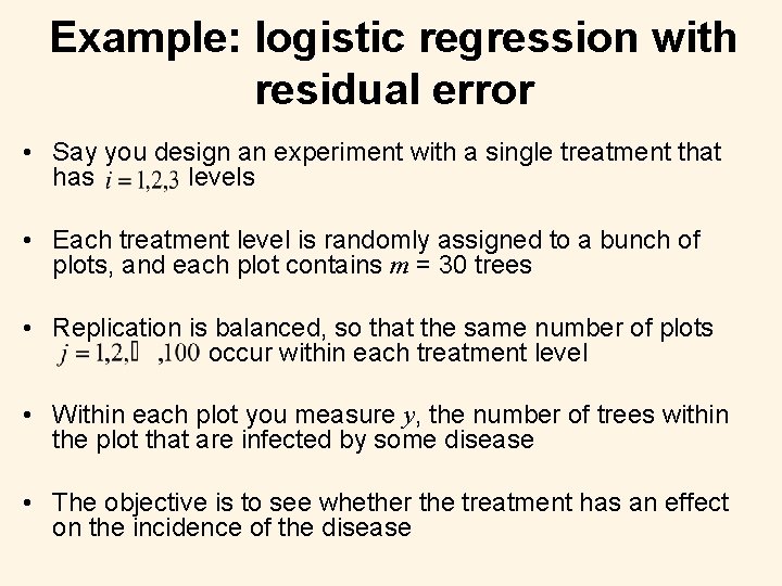
Example: logistic regression with residual error • Say you design an experiment with a single treatment that has levels • Each treatment level is randomly assigned to a bunch of plots, and each plot contains m = 30 trees • Replication is balanced, so that the same number of plots occur within each treatment level • Within each plot you measure y, the number of trees within the plot that are infected by some disease • The objective is to see whether the treatment has an effect on the incidence of the disease

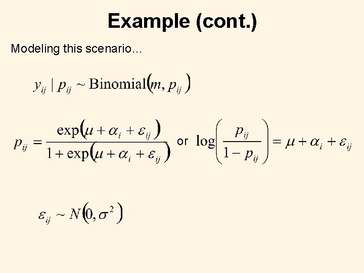
Example (cont. ) Modeling this scenario… or

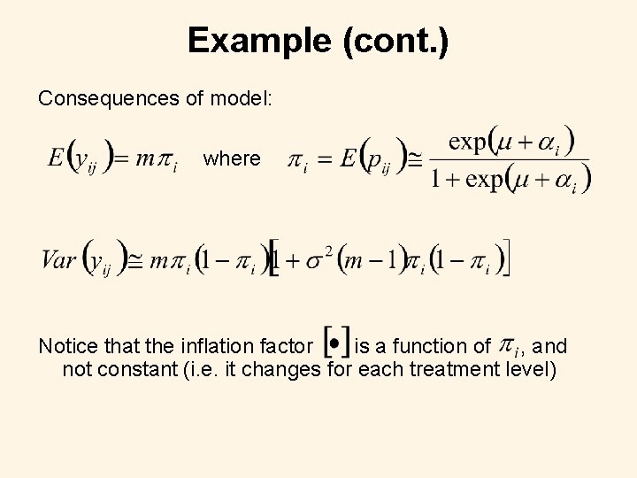
Example (cont. ) Consequences of model: where Notice that the inflation factor is a function of , and not constant (i. e. it changes for each treatment level)

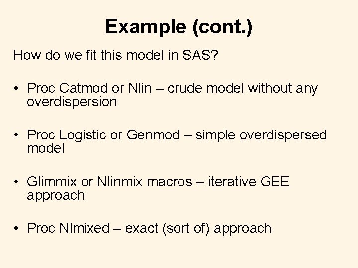
Example (cont. ) How do we fit this model in SAS? • Proc Catmod or Nlin – crude model without any overdispersion • Proc Logistic or Genmod – simple overdispersed model • Glimmix or Nlinmix macros – iterative GEE approach • Proc Nlmixed – exact (sort of) approach

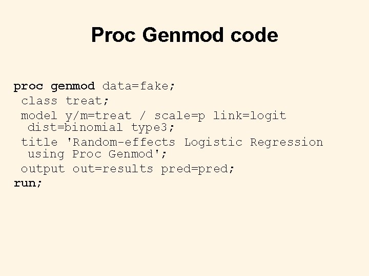
Proc Genmod code proc genmod data=fake; class treat; model y/m=treat / scale=p link=logit dist=binomial type 3; title 'Random-effects Logistic Regression using Proc Genmod'; output out=results pred=pred; run;

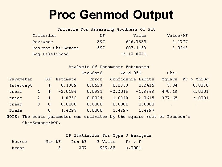
Proc Genmod Output Criteria For Assessing Goodness Of Fit Criterion DF Value Deviance 297 646. 7835 Pearson Chi-Square 297 607. 1128 Log Likelihood -2119. 8941 Value/DF 2. 1777 2. 0442 Analysis Of Parameter Estimates Standard Wald 95% Chi. Parameter DF Estimate Error Confidence Limits Square Pr > Chi. Sq Intercept 1 0. 1389 0. 0523 0. 0363 0. 2415 7. 04 0. 0080 treat 1 1 -2. 0194 0. 0931 -2. 2019 -1. 8368 470. 18 <. 0001 treat 2 1 1. 8726 0. 0964 1. 6838 2. 0615 377. 65 <. 0001 treat 3 0 0. 0000. . Scale 0 1. 4297 0. 0000 1. 4297 NOTE: The scale parameter was estimated by the square root of Pearson's Chi-Square/DOF. Source treat Num DF 2 LR Statistics For Type 3 Analysis Den DF F Value Pr > F 297 929. 55 <. 0001

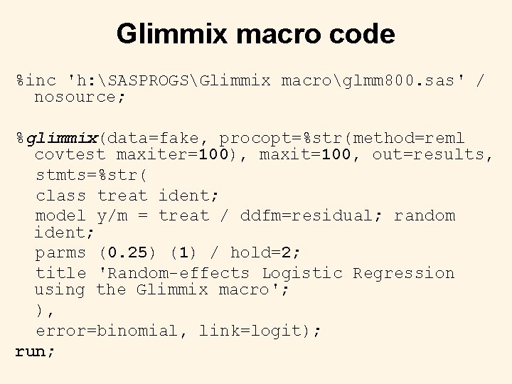
Glimmix macro code %inc 'h: SASPROGSGlimmix macroglmm 800. sas' / nosource; %glimmix(data=fake, procopt=%str(method=reml covtest maxiter=100), maxit=100, out=results, stmts=%str( class treat ident; model y/m = treat / ddfm=residual; random ident; parms (0. 25) (1) / hold=2; title 'Random-effects Logistic Regression using the Glimmix macro'; ), error=binomial, link=logit); run;

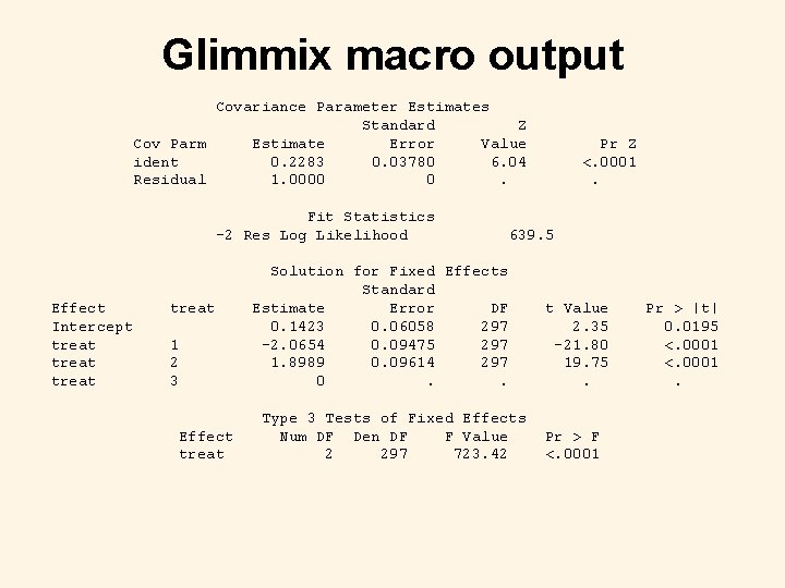
Glimmix macro output Covariance Parameter Estimates Standard Z Cov Parm Estimate Error Value ident 0. 2283 0. 03780 6. 04 Residual 1. 0000 0. Fit Statistics -2 Res Log Likelihood Effect Intercept treat 1 2 3 Effect treat Pr Z <. 0001. 639. 5 Solution for Fixed Effects Standard Estimate Error DF 0. 1423 0. 06058 297 -2. 0654 0. 09475 297 1. 8989 0. 09614 297 0. . Type 3 Tests of Fixed Effects Num DF Den DF F Value 2 297 723. 42 t Value 2. 35 -21. 80 19. 75. Pr > F <. 0001 Pr > |t| 0. 0195 <. 0001.

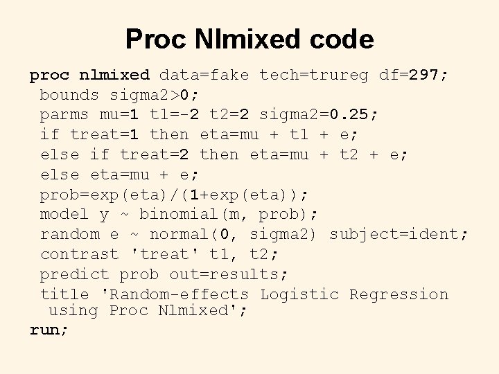
Proc Nlmixed code proc nlmixed data=fake tech=trureg df=297; bounds sigma 2>0; parms mu=1 t 1=-2 t 2=2 sigma 2=0. 25; if treat=1 then eta=mu + t 1 + e; else if treat=2 then eta=mu + t 2 + e; else eta=mu + e; prob=exp(eta)/(1+exp(eta)); model y ~ binomial(m, prob); random e ~ normal(0, sigma 2) subject=ident; contrast 'treat' t 1, t 2; predict prob out=results; title 'Random-effects Logistic Regression using Proc Nlmixed'; run;

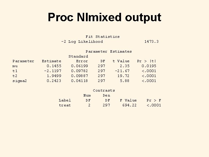
Proc Nlmixed output Fit Statistics -2 Log Likelihood Parameter mu t 1 t 2 sigma 2 Estimate 0. 1455 -2. 1197 1. 9499 0. 2423 1473. 3 Parameter Estimates Standard Error DF t Value 0. 06199 297 2. 35 0. 09782 297 -21. 67 0. 09887 297 19. 72 0. 04118 297 5. 88 Label treat Contrasts Num Den DF DF 2 297 Pr > |t| 0. 0195 <. 0001 F Value 694. 22 Pr > F <. 0001

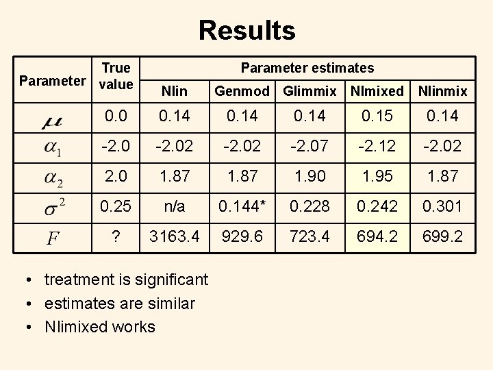
Results True Parameter value F Parameter estimates Nlin Genmod Glimmix Nlmixed Nlinmix 0. 0 0. 14 0. 15 0. 14 -2. 02 -2. 07 -2. 12 -2. 02 2. 0 1. 87 1. 90 1. 95 1. 87 0. 25 n/a 0. 144* 0. 228 0. 242 0. 301 ? 3163. 4 929. 6 723. 4 694. 2 699. 2 • treatment is significant • estimates are similar • Nlimixed works

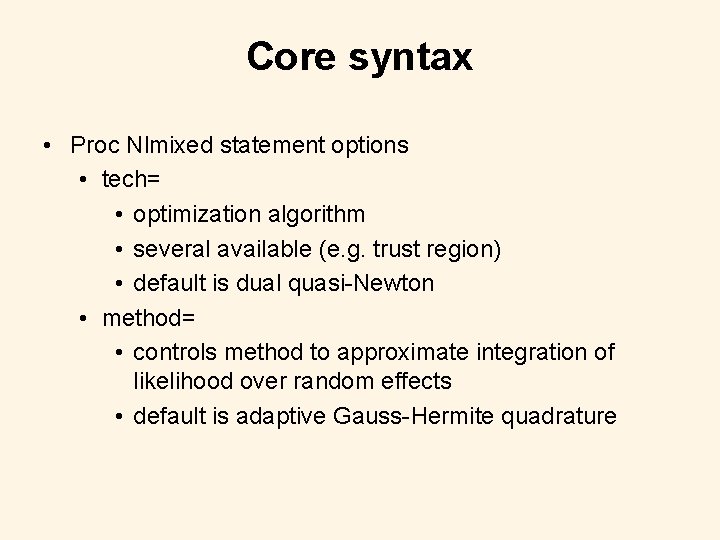
Core syntax • Proc Nlmixed statement options • tech= • optimization algorithm • several available (e. g. trust region) • default is dual quasi-Newton • method= • controls method to approximate integration of likelihood over random effects • default is adaptive Gauss-Hermite quadrature

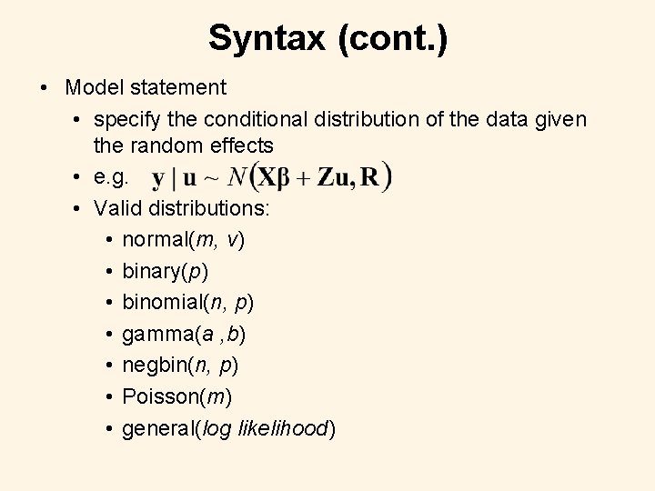
Syntax (cont. ) • Model statement • specify the conditional distribution of the data given the random effects • e. g. • Valid distributions: • normal(m, v) • binary(p) • binomial(n, p) • gamma(a , b) • negbin(n, p) • Poisson(m) • general(log likelihood)

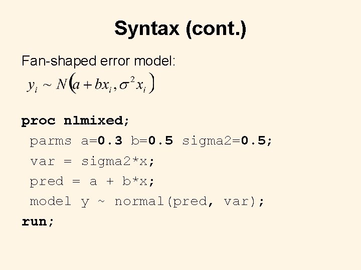
Syntax (cont. ) Fan-shaped error model: proc nlmixed; parms a=0. 3 b=0. 5 sigma 2=0. 5; var = sigma 2*x; pred = a + b*x; model y ~ normal(pred, var); run;

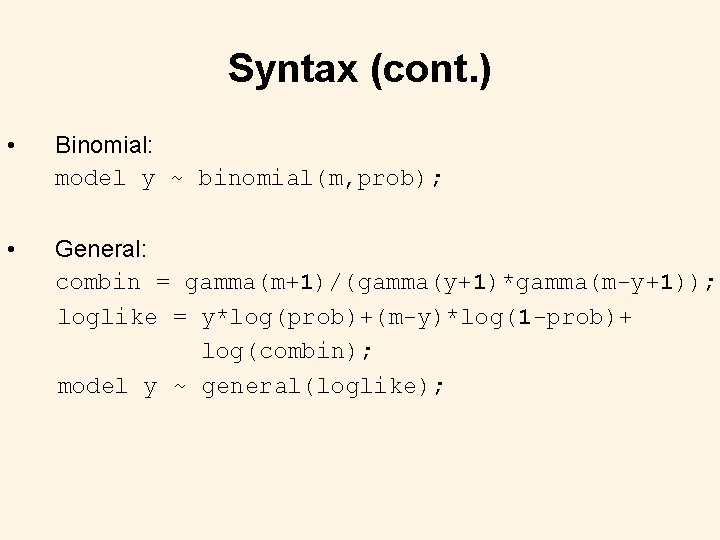
Syntax (cont. ) • Binomial: model y ~ binomial(m, prob); • General: combin = gamma(m+1)/(gamma(y+1)*gamma(m-y+1)); loglike = y*log(prob)+(m-y)*log(1 -prob)+ log(combin); model y ~ general(loglike);

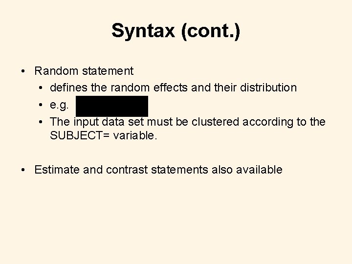
Syntax (cont. ) • Random statement • defines the random effects and their distribution • e. g. • The input data set must be clustered according to the SUBJECT= variable. • Estimate and contrast statements also available

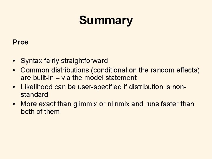
Summary Pros • Syntax fairly straightforward • Common distributions (conditional on the random effects) are built-in – via the model statement • Likelihood can be user-specified if distribution is nonstandard • More exact than glimmix or nlinmix and runs faster than both of them

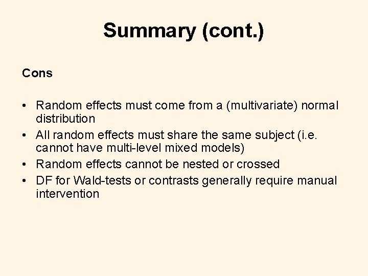
Summary (cont. ) Cons • Random effects must come from a (multivariate) normal distribution • All random effects must share the same subject (i. e. cannot have multi-level mixed models) • Random effects cannot be nested or crossed • DF for Wald-tests or contrasts generally require manual intervention

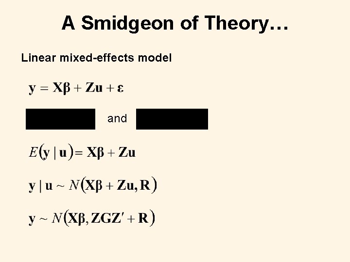
A Smidgeon of Theory… Linear mixed-effects model and

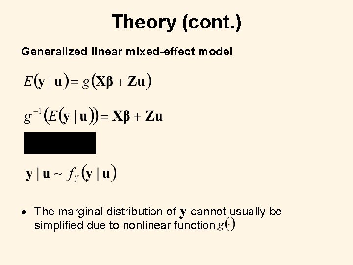
Theory (cont. ) Generalized linear mixed-effect model The marginal distribution of y cannot usually be simplified due to nonlinear function

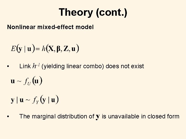
Theory (cont. ) Nonlinear mixed-effect model • Link h-1 (yielding linear combo) does not exist • The marginal distribution of y is unavailable in closed form

Conclusion • Flexibility of proc nlmixed makes it a good choice for many non-standard applications (e. g. non-linear models), even those without random effects.

References • Huet, S. , Bouvier, A. , Poursat, M. -A. , and E. Jolivet. 2004. Statistical Tools for Nonlinear Regression. A Practical Guide with S-PLUS and R Examples, Second Edition. Springer-Verlag. New York. • Littell, R. C. , Milliken, G. A. , Stroup, W. W. , and R. D. Wolfinger. 1996. SAS System for Mixed Models. Cary, NC. SAS Institute Inc. • Mc. Cullogh, C. E. and S. R. Searle. 2001. Generalized, Linear, and Mixed Models. John Wiley & Sons. New York • Pinheiro, J. C. and D. M. Bates. 2000. Mixed-effects Models in S and S -PLUS. Springer-Verlag. New York. • SAS Institute Inc. 2004. SAS Online. Doc® 9. 1. 3. Cary, NC: SAS Institute Inc.