The Power Flow Problem Scott Norr For EE

The Power Flow Problem Scott Norr For EE 4501 April, 2015

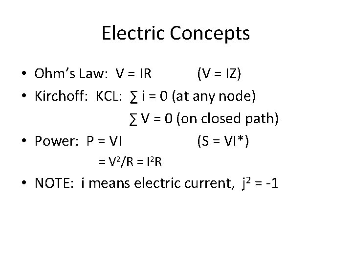
Electric Concepts • Ohm’s Law: V = IR (V = IZ) • Kirchoff: KCL: ∑ i = 0 (at any node) ∑ V = 0 (on closed path) • Power: P = VI (S = VI*) = V 2/R = I 2 R • NOTE: i means electric current, j 2 = -1

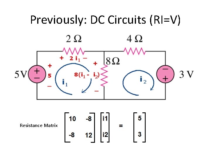
Previously: DC Circuits (RI=V) Resistance Matrix

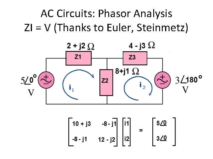
AC Circuits: Phasor Analysis ZI = V (Thanks to Euler, Steinmetz) Impedance Matrix

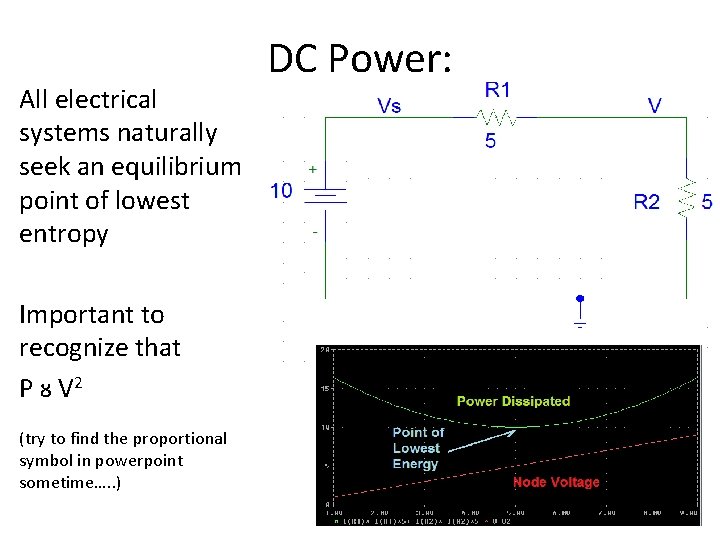
All electrical systems naturally seek an equilibrium point of lowest entropy Important to recognize that P ᴕ V 2 (try to find the proportional symbol in powerpoint sometime…. . ) DC Power:

AC Power • The complex power, S = VI* = P + j. Q • P is the average power (“real” power) in watts, attributable to resistive loads • Q is the reactive power (“imaginary” power) in VAr, attributable to capacitive and inductive loads

The Power Problem: • On AC power systems, we don’t predetermine the phase angles on the sources, they are determined by the system (additional unknowns to solve for!) • Power is injected into nodes in the system via sources and is removed at nodes via loads (consumption points) • Additionally, power is lost in the network

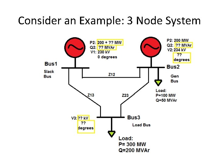
Consider an Example: 3 Node System

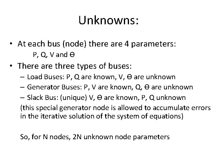
Unknowns: • At each bus (node) there are 4 parameters: P, Q, V and Ө • There are three types of buses: – Load Buses: P, Q are known, V, Ө are unknown – Generator Buses: P, V are known, Q, Ө are unknown – Slack Bus: (unique) V, Ө are known, P, Q unknown (this special generator node is allowed to accumulate errors in the iterative solution of the system of equations) So, for N nodes, 2 N unknown node parameters

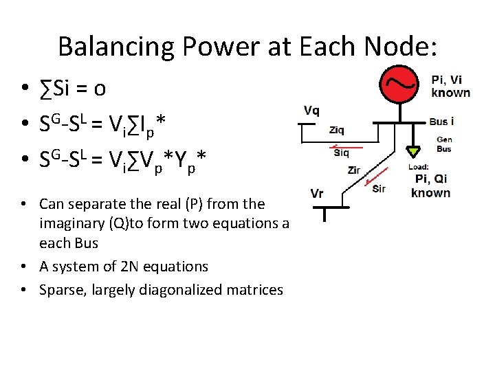
Balancing Power at Each Node: • ∑Si = o • SG-SL = Vi∑Ip* • SG-SL = Vi∑Vp*Yp* • Can separate the real (P) from the imaginary (Q)to form two equations at each Bus • A system of 2 N equations • Sparse, largely diagonalized matrices

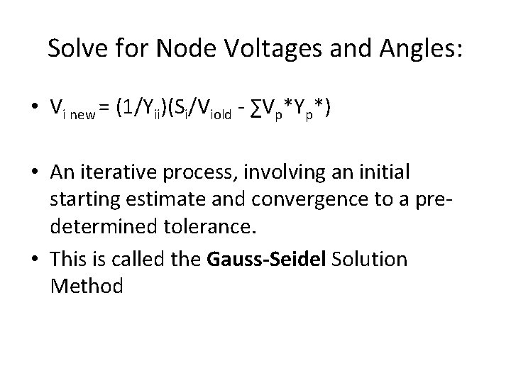
Solve for Node Voltages and Angles: • Vi new = (1/Yii)(Si/Viold - ∑Vp*Yp*) • An iterative process, involving an initial starting estimate and convergence to a predetermined tolerance. • This is called the Gauss-Seidel Solution Method

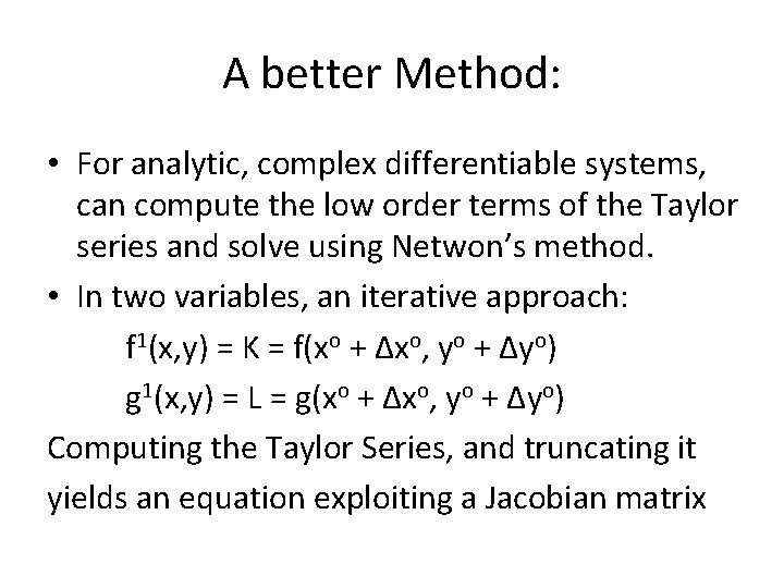
A better Method: • For analytic, complex differentiable systems, can compute the low order terms of the Taylor series and solve using Netwon’s method. • In two variables, an iterative approach: f 1(x, y) = K = f(xo + Δxo, yo + Δyo) g 1(x, y) = L = g(xo + Δxo, yo + Δyo) Computing the Taylor Series, and truncating it yields an equation exploiting a Jacobian matrix

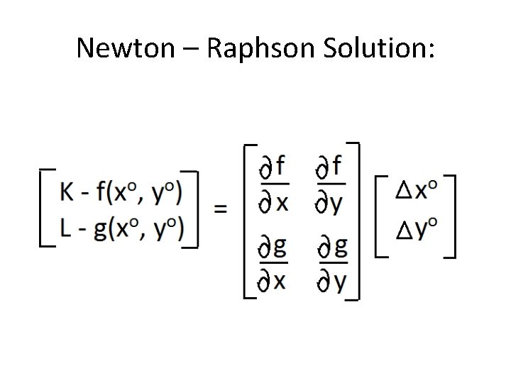
Newton – Raphson Solution:

Conclusions: • Powerflow Software is used by every electric utility in the world. Many models contain 10, 000 nodes or more. • There are quite a few solution techniques that are more efficient than the G-S and N-R methods outlined here: Fast-Decoupled N-R – decouples P, O from Q, V and solves the two, smaller systems Interior Point Newton - calculates a Hessian Mtx!

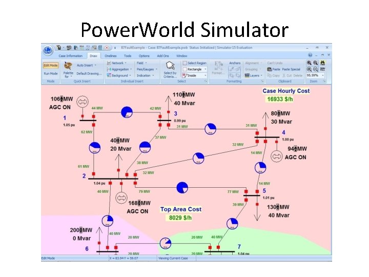
Power. World Simulator

References: • Stevenson, William D. , Elements of Power System Analysis, Mc. Graw-Hill, 1982 • Tylavsky, Daniel, Lecture Notes #19, EEE 574, Arizona State University, 1999 • Power. World Simulator, www. powerworld. com, 2014