The Polynomial Hierarchy And Randomized Computations Complexity D

The Polynomial Hierarchy And Randomized Computations Complexity ©D. Moshkovitz 1

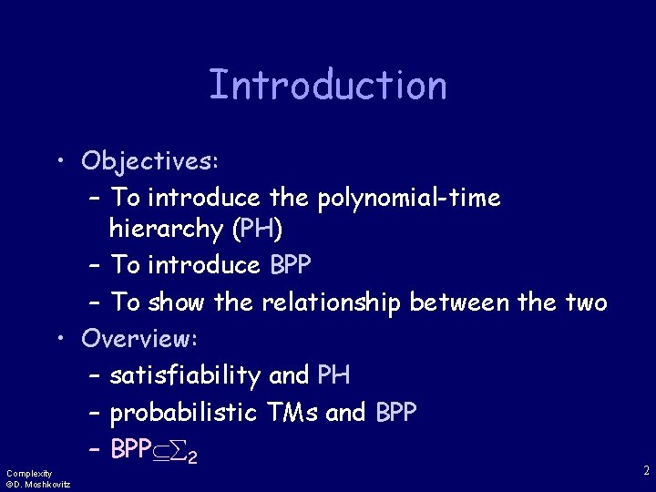
Introduction • Objectives: – To introduce the polynomial-time hierarchy (PH) – To introduce BPP – To show the relationship between the two • Overview: – satisfiability and PH – probabilistic TMs and BPP – BPP 2 Complexity ©D. Moshkovitz 2

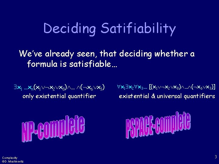
Deciding Satifiability We’ve already seen, that deciding whether a formula is satisfiable… x 1 …xn(x 1 x 2 x 8) … ( x 6 x 3) only existential quantifier Complexity ©D. Moshkovitz x 1 x 2 x 3… [(x 1 x 2 x 8) … ( x 6 x 3)] existential & universal quantifiers 3

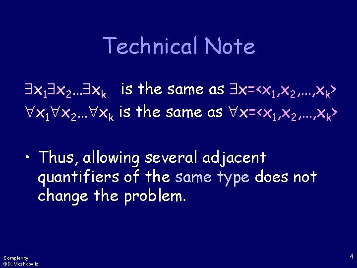
Technical Note x 1 x 2… xk is the same as x=<x 1, x 2, …, xk> • Thus, allowing several adjacent quantifiers of the same type does not change the problem. Complexity ©D. Moshkovitz 4

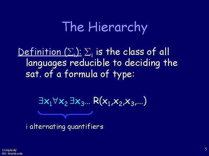
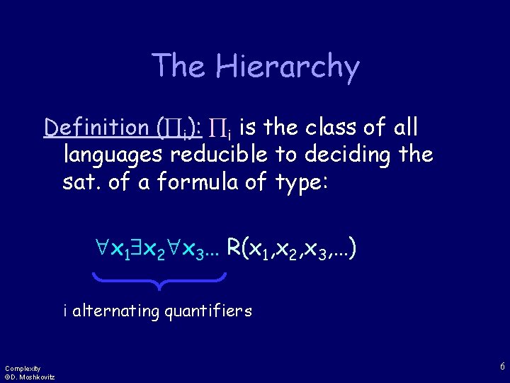
The Hierarchy Definition ( i): i is the class of all languages reducible to deciding the sat. of a formula of type: x 1 x 2 x 3… R(x 1, x 2, x 3, …) i alternating quantifiers Complexity ©D. Moshkovitz 5

The Hierarchy Definition ( i): i is the class of all languages reducible to deciding the sat. of a formula of type: x 1 x 2 x 3… R(x 1, x 2, x 3, …) i alternating quantifiers Complexity ©D. Moshkovitz 6

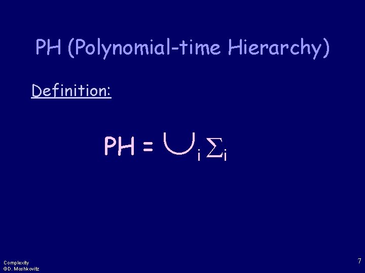
PH (Polynomial-time Hierarchy) Definition: PH = Complexity ©D. Moshkovitz i i 7

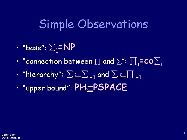
Simple Observations • “base”: 1=NP i=co i “hierarchy”: i i+1 and i i+1 “upper bound”: PH PSPACE • “connection between and ”: • • Complexity ©D. Moshkovitz 8

Can the Hierarchy Collapse? Proposition: If NP=co. NP, then PH=NP. Proof Idea: By induction on i, i=NP. Complexity ©D. Moshkovitz 9

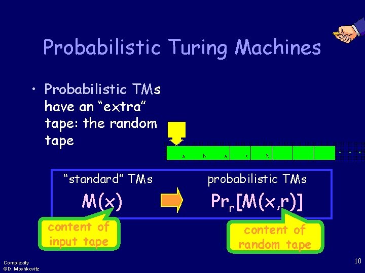
Probabilistic Turing Machines • Probabilistic TMs have an “extra” tape: the random tape “standard” TMs M(x) content of input tape Complexity ©D. Moshkovitz probabilistic TMs Prr[M(x, r)] content of random tape 10

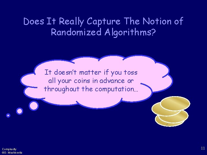
Does It Really Capture The Notion of Randomized Algorithms? It doesn’t matter if you toss all your coins in advance or throughout the computation… Complexity ©D. Moshkovitz 11

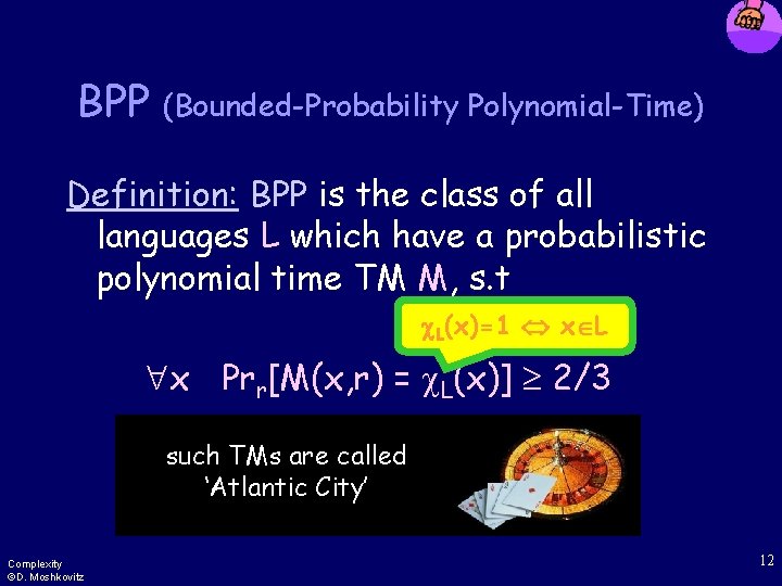
BPP (Bounded-Probability Polynomial-Time) Definition: BPP is the class of all languages L which have a probabilistic polynomial time TM M, s. t L(x)=1 x L x Prr[M(x, r) = L(x)] 2/3 such TMs are called ‘Atlantic City’ Complexity ©D. Moshkovitz 12

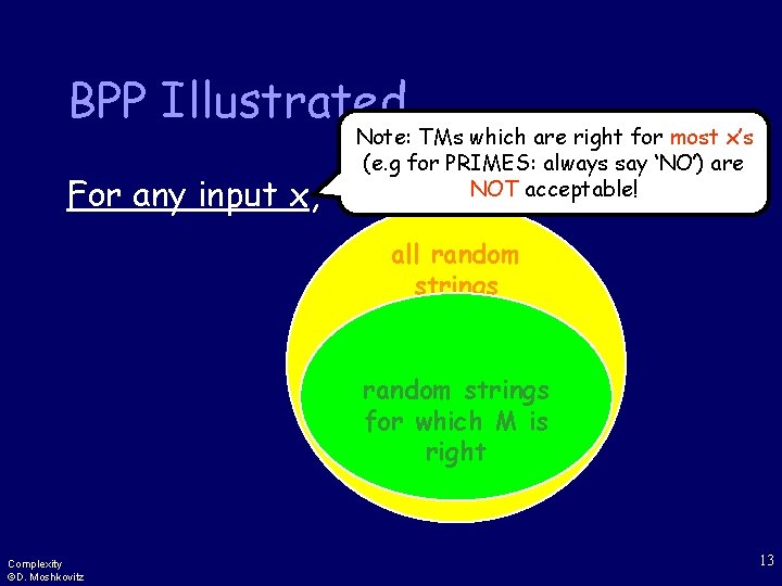
BPP Illustrated For any input x, Note: TMs which are right for most x’s (e. g for PRIMES: always say ‘NO’) are NOT acceptable! all random strings for which M is right Complexity ©D. Moshkovitz 13

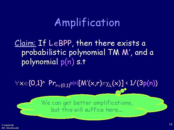
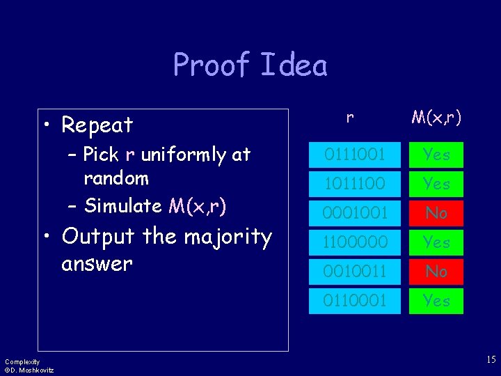
Amplification Claim: If L BPP, then there exists a probabilistic polynomial TM M’, and a polynomial p(n) s. t x {0, 1}n Prr {0, 1}p(n)[M’(x, r) L(x)] < 1/(3 p(n)) We can get better amplifications, but this will suffice here. . . Complexity ©D. Moshkovitz 14

Proof Idea • Repeat – Pick r uniformly at random – Simulate M(x, r) • Output the majority answer Complexity ©D. Moshkovitz r M(x, r) 0111001 Yes 1011100 Yes 0001001 No 1100000 Yes 0010011 No 0110001 Yes 15

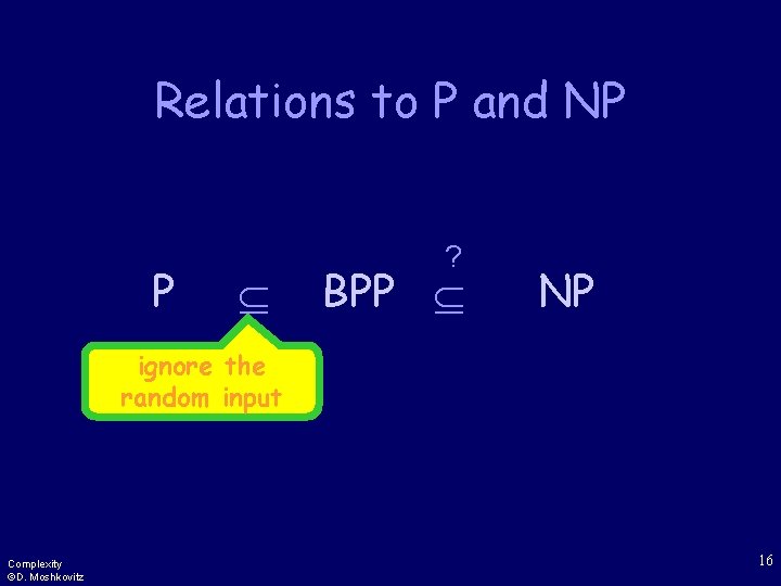
Relations to P and NP P ? BPP NP ignore the random input Complexity ©D. Moshkovitz 16

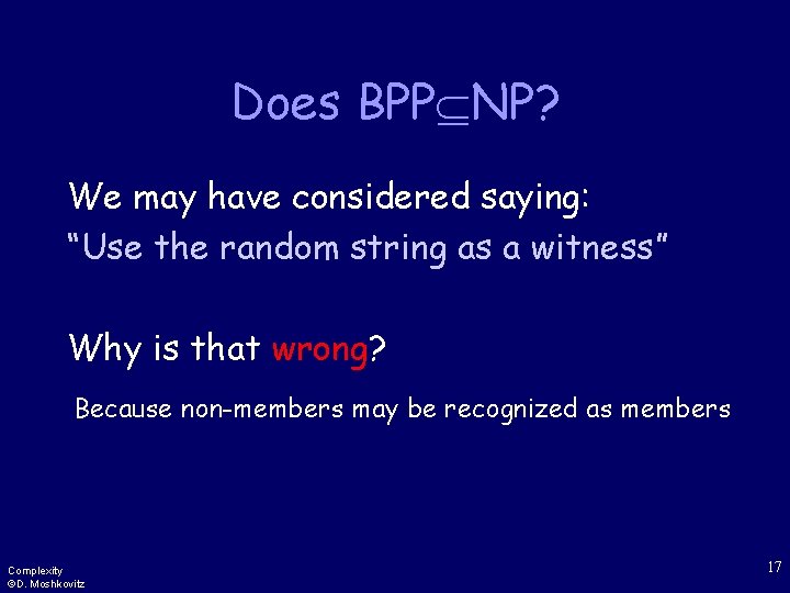
Does BPP NP? We may have considered saying: “Use the random string as a witness” Why is that wrong? Because non-members may be recognized as members Complexity ©D. Moshkovitz 17

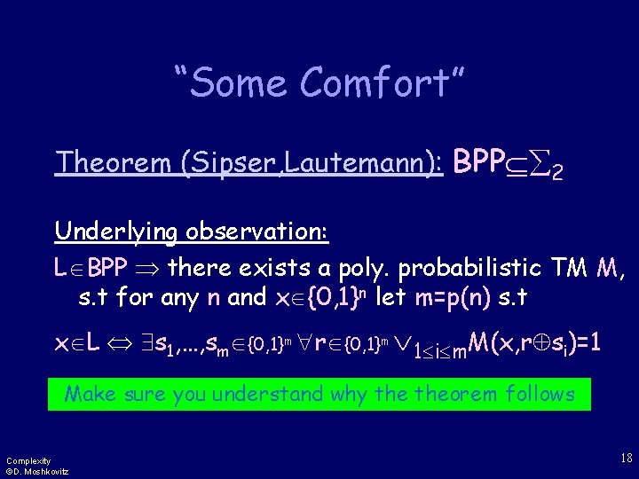
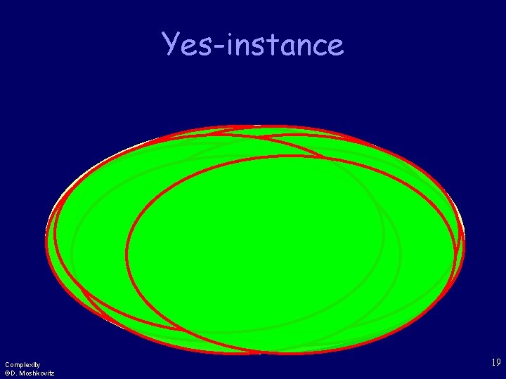
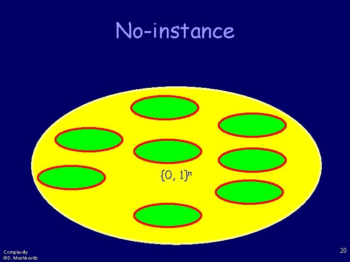
“Some Comfort” Theorem (Sipser, Lautemann): BPP 2 Underlying observation: L BPP there exists a poly. probabilistic TM M, s. t for any n and x {0, 1}n let m=p(n) s. t x L s 1, …, sm {0, 1}m r {0, 1}m 1 i m. M(x, r si)=1 Make sure you understand why theorem follows Complexity ©D. Moshkovitz 18

Yes-instance {0, 1}n Complexity ©D. Moshkovitz 19

No-instance {0, 1}n Complexity ©D. Moshkovitz 20

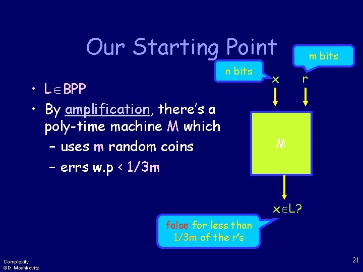
Our Starting Point n bits • L BPP • By amplification, there’s a poly-time machine M which – uses m random coins – errs w. p < 1/3 m x m bits r M x L? false for less than 1/3 m of the r’s Complexity ©D. Moshkovitz 21

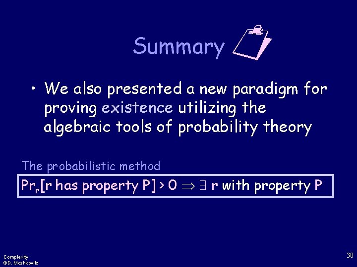
Proving the Underlying Observation We will follow the Probabilistic Method Prr[r has property P] > 0 r with property P Complexity ©D. Moshkovitz 22

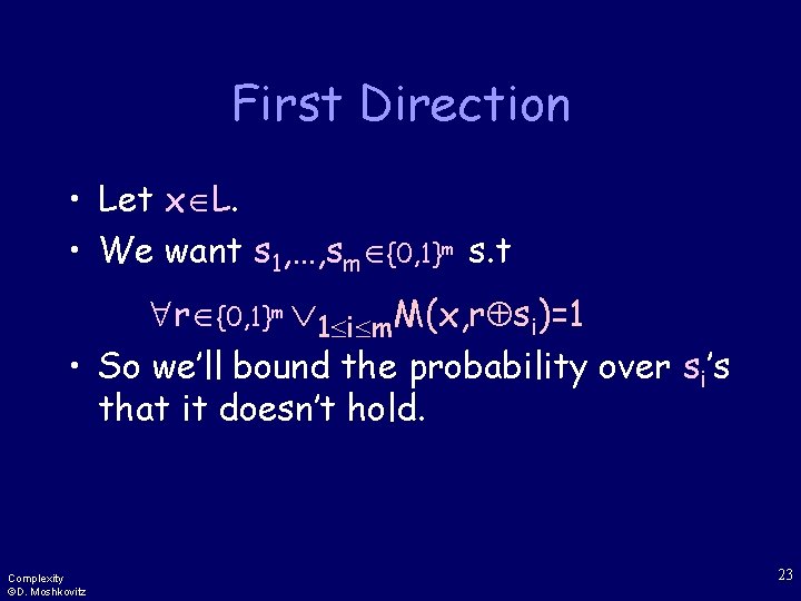
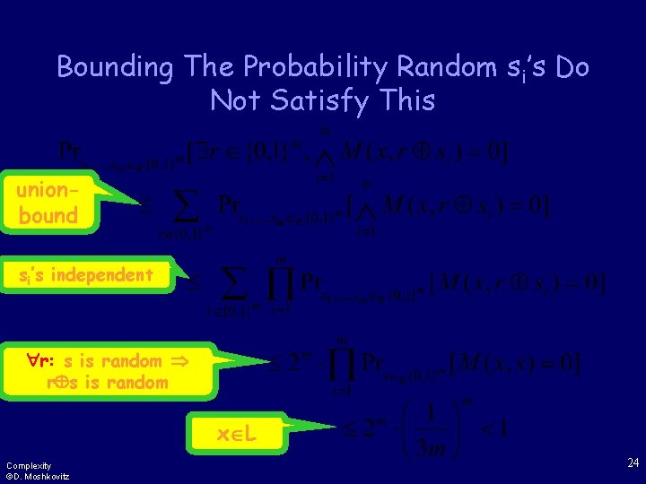
First Direction • Let x L. • We want s 1, …, sm {0, 1}m s. t r {0, 1}m 1 i m. M(x, r si)=1 • So we’ll bound the probability over si’s that it doesn’t hold. Complexity ©D. Moshkovitz 23

Bounding The Probability Random si’s Do Not Satisfy This unionbound si’s independent r: s is random r s is random x L Complexity ©D. Moshkovitz 24

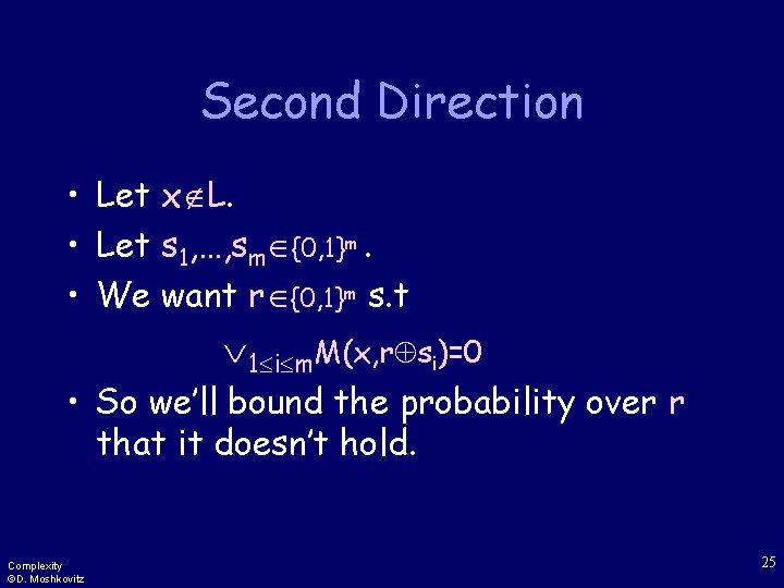
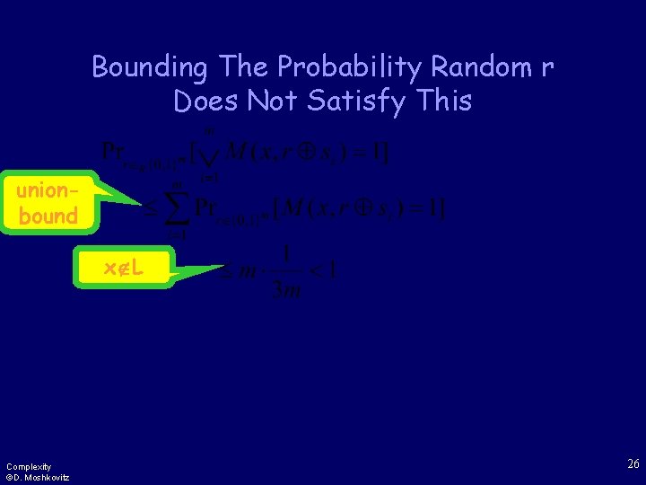
Second Direction • Let x L. • Let s 1, …, sm {0, 1}m. • We want r {0, 1}m s. t 1 i m. M(x, r si)=0 • So we’ll bound the probability over r that it doesn’t hold. Complexity ©D. Moshkovitz 25

Bounding The Probability Random r Does Not Satisfy This unionbound x L Complexity ©D. Moshkovitz 26

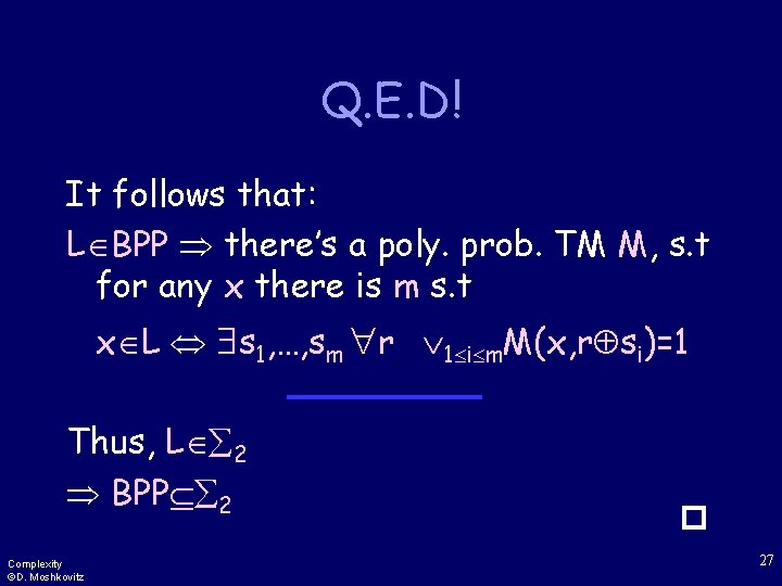
Q. E. D! It follows that: L BPP there’s a poly. prob. TM M, s. t for any x there is m s. t x L s 1, …, sm r 1 i m. M(x, r si)=1 Thus, L 2 BPP 2 Complexity ©D. Moshkovitz 27

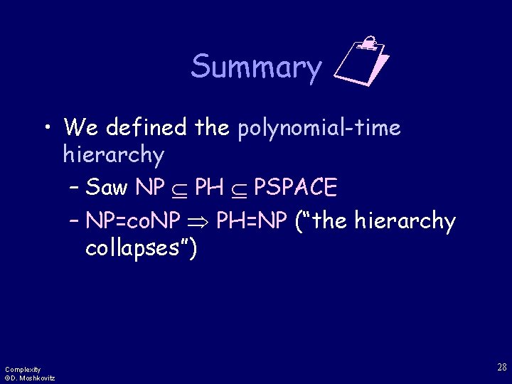
Summary • We defined the polynomial-time hierarchy – Saw NP PH PSPACE – NP=co. NP PH=NP (“the hierarchy collapses”) Complexity ©D. Moshkovitz 28

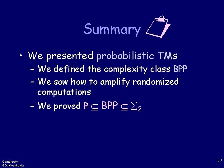
Summary • We presented probabilistic TMs – We defined the complexity class BPP – We saw how to amplify randomized computations – We proved P BPP 2 Complexity ©D. Moshkovitz 29

Summary • We also presented a new paradigm for proving existence utilizing the algebraic tools of probability theory The probabilistic method Prr[r has property P] > 0 r with property P Complexity ©D. Moshkovitz 30