The Periodic Table See Shankar pp 369 371

The Periodic Table (See Shankar pp. 369 -371, Griffiths sect. 5. 2. 2) Understanding the periodic table is one fo the triumphs of QM. Recall that for hydrogen, the electron energy eigenstates are |n, l, m>, where n=1, 2, 3, … l=0, 1, …, n-1 m=-I, …, 0, …, l n=principal quantum number, l=orbital quantum number, m=azimuthal (or magnetic) quantum number. At a given energy-level n, there are n 2 degenerate states. Note too that since the electron is a spin-1/2 fermion, it can be in a spin-up or spin-down state of Sz. So the electron’s state can be further specified by its spin quantum number ms = +1/2 or -1/2. Hence, the degeneracy at energy level n, including electron spin, is 2 n 2. Spectroscopic notation: l=0 s, l=1 p, l=2 d, l=3 f, … (So, for example, a 2 p state refers to the state n=2, l=1. ) Thus, the eigenstates (i. e. orbitals) for the electron are 1 s, 2 p, 3 s, 3 p, 3 d, ….

Understanding Multi-electron atoms The basic picture follows from some simple considerations/approximations 1) Crudest approximation: ignore all electron-electron interactions! So each electron is in one of the hydrogenic (i. e. , single-electron) eigenstates (called “orbitals”) 2) Pauli exclusion principle: no two electrons can occupy the same exact state 3) Electrons fill orbitals in order of increasing energy 4) Electron-electron interactions break the degeneracy in l of hydrogen: For a given n, states with higher l values tend to have higher energy (since higher l means more angular momentum, and such an electron tends to be farther from the nucleus and hence the inner electrons tend to “shield” the nucleus. 5) States with filled shells (i. e. , n-levels) or filled subshells (i. e. , subshells) tend to be chemically inert, since the total electric charge configuration is spherically symmetric, so they shield their nucleus effectively, and hence there is little electron affinity for electrons in other atoms. With this in mind, we can now construct the expected ground states of various elements …

Element 1 s 2 s 2 p 2 p 2 p Electron configuration H (1 s)1 He (1 s)2 Li (1 s)2(2 s)1 Be (1 s)2(2 s)2 B (1 s)2(2 p)1 C (1 s)2(2 p)2 N (1 s)2(2 p)3 O (1 s)2(2 p)4 F (1 s)2(2 p)5 Ne (1 s)2(2 p)6

Notice that He, Ne, Ar, Kr, . . . making up the last column of the periodic table tend to be chemically inert. Elements in the first column, such as Li, Na, … have one “extra” electron, so to speak. This extra electron “sees” a net charge of only +e when it “looks inward”, since the 10 inner electrons effectively “screen” much of the +11 e nucleus – i. e. , the outer electron in Na is only loosely bound to the atom. Thus, Na is fairly willing to give up this loosely bound “valence” electron to other atoms. Elements in the column next to the noble gas column, such as F, Cl, …”want” to receive an extra electron. So Na and F make a good match: Na will donate an electron to F, in which case both atoms are ionized, and thus held together by an “ionic bond. ” As we continue along the periodic table, some of our preceding rules must be modified. For example, after argon Ar= (Ne)(3 s)2(3 p)6 comes potassium K =(Ar)(4 s). Notice that we would have expected potassium’s 19 th electron to go into the 3 d state, not the 4 s state. Why didn’t it? Because the growth in energy due to the increase in l is larger than the increase in energy from n=3 to n=4, so it is energetically favorable for the extra electron to go into the 4 s state!

Addition of Angular Momentum Reading: Shankar chapt. 15 and Griffiths 4. 4. 3 We found that the angular-momentum state of a particle (either orbital or spin) could be represented by |j, m>, where j, m are “good quantum numbers” associated with the operators J 2, Jz: Here, “good” means that these numbers can be simultaneously specified, since the two operators commute. And of course we also determined commutation relations involving other related operators, including Jx Jy, Jz J 2, J+, J-.

If we have either a) 2 (or more) distinct particles, each with its own angular momentum, such as in a multi-electron atom b) A single particle that has both orbital and spin angular momentum, such as the electron of a hydrogen atom Then we can ask questions about what the total angular momentum of the system is. Preliminaries Start with 2 angular momenta assume they commute): belonging to different subspaces (i. e. ,

The state of the composite system is given by (equivalent notation: In this uncoupled representation, the system is specified by 4 quantum numbers, -- i. e. , the operators form a complete set of commuting observables! (Note: the dimensionality of the composite system is just the product of the dimensionality of the two subspaces). The above representation is a perfectly good way of expressing the angular momentum state of the composite system. We now look at an alternative means of doing this which proves especially useful.

Total angular momentum Define the total angular momentum The magnitude and z-component of the total angular momentum for the composite system is described by operators Do these operators commute with one another? --YES (Stop and verify this for yourself!) So these operators share a common set of eigenvectors, and thus they provide us with two good quantum numbers. We’ll call these j and m, and denote the eigenstate |j, m>. Since the total angular momentum is still just an angular momentum, by earlier arguments we have

where m = -j, -j+1, … 0, …, j-1, j But wait! In the uncoupled representation, the angular momentum of the composite system is specified by 4 good quantum numbers. But so far, in terms of the total angular momentum, we have only found 2 good quantum numbers: j, associated with the magnitude of the total angular momentum, and m, associated with the z-component of the total angular momentum. We’ll need to hunt around for (two) additional operators that commute with one another and with I’ll spare you the search: Let’s do a quick, partial verification of this.

(Verify for yourself, for example, that J 2 doesn’t commute with J 1 z or with J 2 z) We’ll call the representation in which coupled representation, and denote the eigenstates by are specified the In the coupled representation, we have the obvious (or at least plausible) relations:

Relation between representations So we have two perfectly good bases for describing the angular momentum of a composite system: What’s the relation between the two? themselves. Let’s start with the quantum numbers Now, since the max value of m 1 is j 1, and since the max value of m 2 is j 2, it follows that mmax=j 1+j 2. But we also know that m ranges from –j, …, j. Hence we can conclude that jmax=j 1+j 2. (Perhaps this isn’t surprising: classically, the magnitude of the total angular momentum of a composite system can’t exceed that of its individual components.

Reasoning classically, we might also anticipate that there is a minimum value of j for the composite system, given by the difference |j 1 -j 2| (corresponding to when the angular momentum of the individual components of the system point in opposite directions). This is indeed the case, as we now show using a counting argument: For a given j 1, j 2, there a total of (2 j 1+1)(2 j 2+1) independent basis vectors of the form |j 1, m 1> |j 2, m 2>. This must be the same total as for the |j, m, j 1, j 2> basis (with j 1, j 2 fixed as before). Now, for each j, there are (2 j+1) possible m values. So we demand that

Summarizing, Now let’s compute the relationship between the basis vectors of the coupled and uncoupled representations: The coefficients are called the Clebsch-Gordan coefficients. Their interpretation is straightforward: gives the probability that, for a specified j and m, a measurement of j 1 z will yield the value m 1 and a measurement of j 2 z will yield the value m 2.

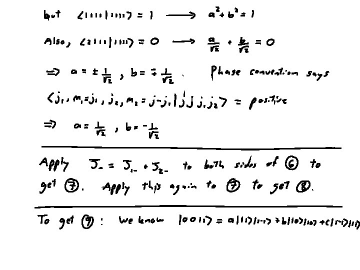
Calculation of the Clebsch-Gordan coefficients can be done by appropriate application of the raising/lowering operators J+, J- (though we note that these calculations tend to be tedious, so look-up tables exist to assist you). [Note: The standard phase convention used when defining basis vectors |j, m, j 1, j 2> is such that all Clebsch-Gordan coefficients are purely real, and that the projection <j 1, m 1=j 1; j 2, m 2=j-j 1 | j, m, j 1, j 2> is real. ] Here’s an example calculation: What does the state |1, -1, 1, 1> look like in the uncoupled representation?

It’s easy to find the Clebsch-Gordan coefficients in two limiting cases: 1) 2) If you’re interested in a general way of calculating Clebsch-Gordan coefficients, the following (recursion) relation proves useful:

Equating these two expressions leads to a useful relation that allows one to (recursively) generate all Clebsch-Gordan coefficients (provided one uses the orthogonality conditions as well). Example 1: The allowed (m 1, m 2) and (j, m) values if j 1=1 and j 2=3/2 m 1 m 2 m j Notes: a) There are 12 distinct combinations of (m 1, m 2), and 12 distinct combo’s of (j, m) b) Table is organized by decreasing m values.

Example 2: Two spin ½ particles

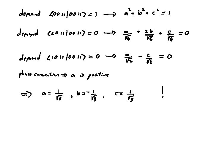
Example 3: Angular momentum of two p electrons (i. e. , j 1=1 and j 2=1).

To show this, will need plus orthogonality relations (plus phase choice)