The North Atlantic Meridional Overturning Circulation A system

The North Atlantic Meridional Overturning Circulation – A system with a potential threshold response Guest Lecture Klaus Keller Department of Geosciences, Penn State klaus@psu. edu 1

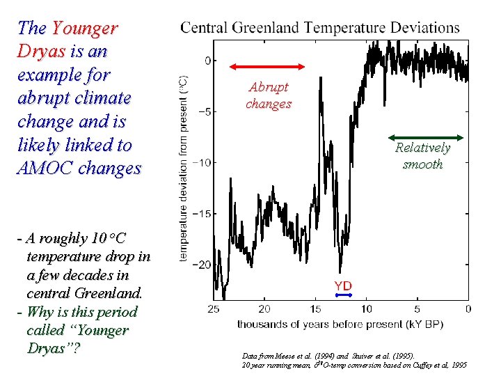
The Younger Dryas is an example for abrupt climate change and is likely linked to AMOC changes - A roughly 10 o. C temperature drop in a few decades in central Greenland. - Why is this period called “Younger Dryas”? Abrupt changes Relatively smooth Data from Meese et al. (1994) and Stuiver et al. (1995). 20 year running mean, d 18 O-temp conversion based on Cuffey et al, 1995

The Younger Dryas is named after the dominance of the pollen of the arctic wildflower Dryas octopetala. Was the Younger Dryas a global climate event? http: //en. wikipedia. org/wiki/Dryas_octopetala

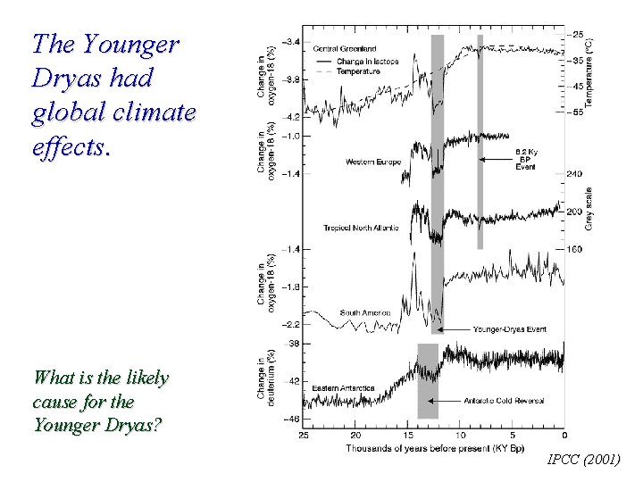
The Younger Dryas had global climate effects. What is the likely cause for the Younger Dryas? IPCC (2001)

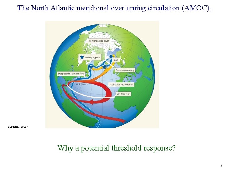
The North Atlantic meridional overturning circulation (AMOC). Quadfasel (2006) Why a potential threshold response? 5

What is a climate threshold? - A negative feedback loop switches signs. - The response can occur faster than the forcing and show hysteresis. - Abruptness and hysteresis can amplify the marginal impacts of forcings that trigger the threshold response. - An actionable early warning sign (before the forcing threshold is crossed) may be of considerable economic value. How does this apply to the AMOC? 6

What mechanism could explain a relatively stable MOC? One key negative (stabilizing) feedback: MOC Advection SST MOC modified from Stocker et al (2001) 7

What mechanism could explain a potential threshold response of the MOC? One key positive (destabilizing) feedback: MOC Advection SSS MOC modified from Stocker et al (2001) 8

What mechanism could explain a potential AMOC threshold response to anthropogenic climate forcings? modified from Stocker et al (2001) 9

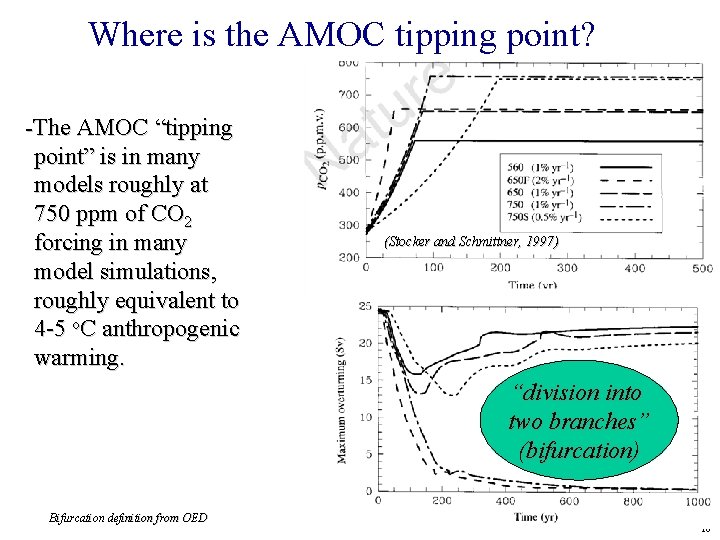
Where is the AMOC tipping point? -The AMOC “tipping point” is in many models roughly at 750 ppm of CO 2 forcing in many model simulations, roughly equivalent to 4 -5 o. C anthropogenic warming. (Stocker and Schmittner, 1997) “division into two branches” (bifurcation) Bifurcation definition from OED 10

Current MOC projections are deeply uncertain. IPCC FAR WG 1 Figure 10. 15 11

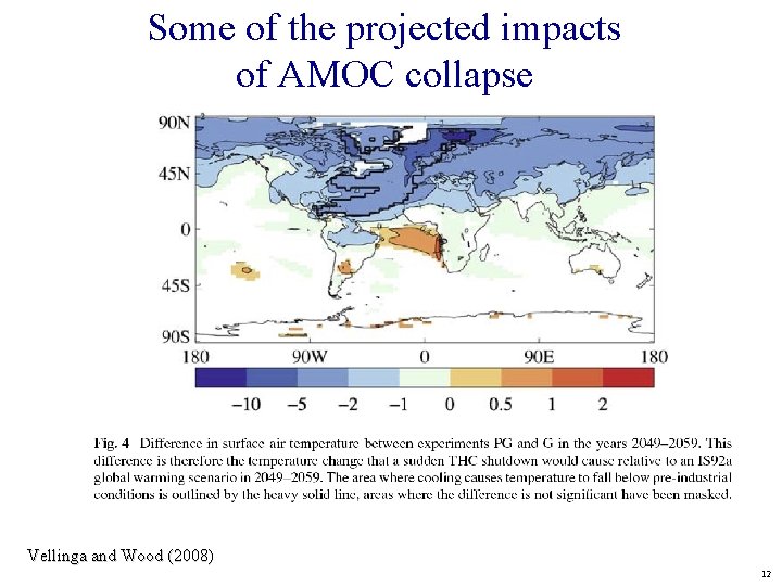
Some of the projected impacts of AMOC collapse Vellinga and Wood (2008) 12

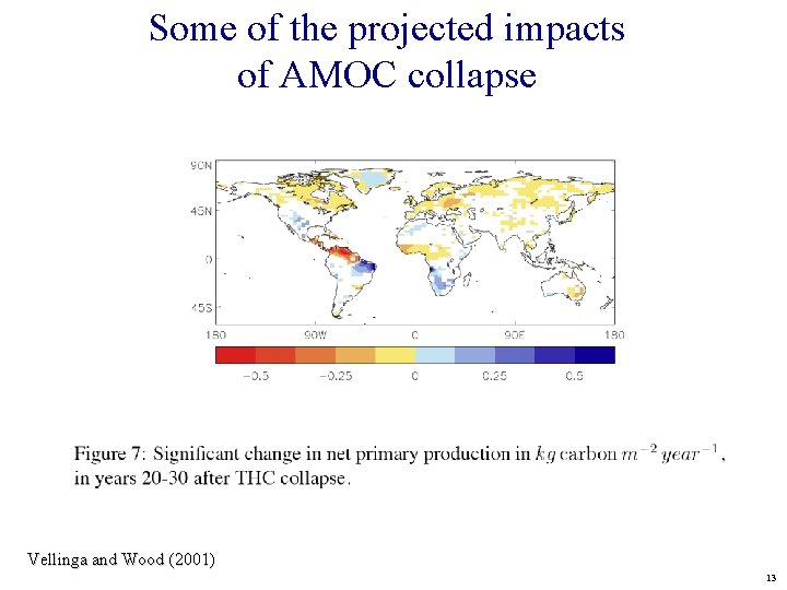
Some of the projected impacts of AMOC collapse Vellinga and Wood (2001) 13

Reserve Materials 14

(2) Would we see threshold coming early enough http: //libweb 5. princeton. edu/Visual_Materials/gallery/animation/ TM - © 1997 - Warner Bros. 15

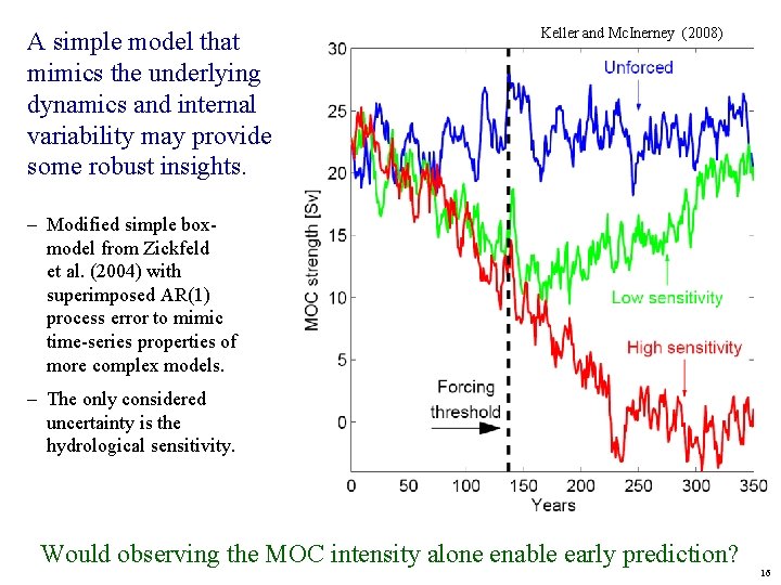
A simple model that mimics the underlying dynamics and internal variability may provide some robust insights. Keller and Mc. Inerney (2008) – Modified simple boxmodel from Zickfeld et al. (2004) with superimposed AR(1) process error to mimic time-series properties of more complex models. – The only considered uncertainty is the hydrological sensitivity. Would observing the MOC intensity alone enable early prediction? 16

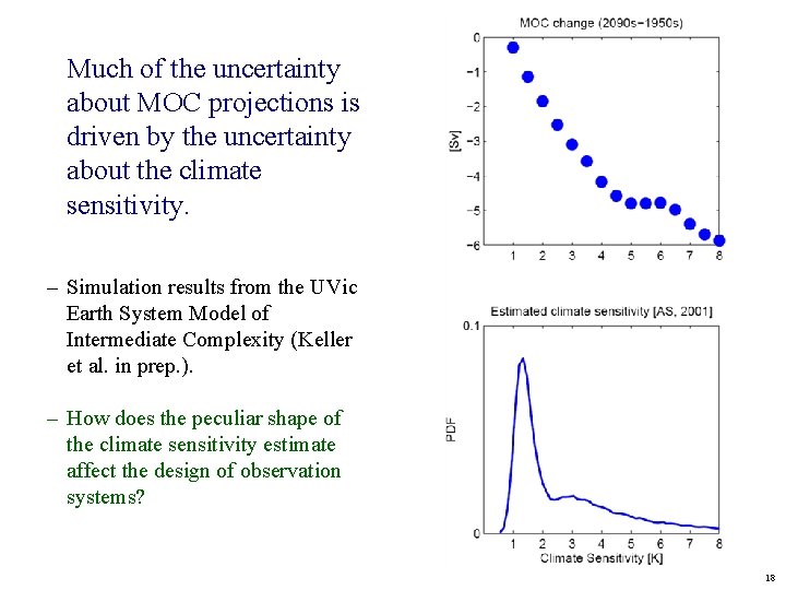
What are key drivers of MOC projection uncertainty? How sensitive are the projected MOC changes to the uncertainty about the climate sensitivity? 17

Much of the uncertainty about MOC projections is driven by the uncertainty about the climate sensitivity. – Simulation results from the UVic Earth System Model of Intermediate Complexity (Keller et al. in prep. ). – How does the peculiar shape of the climate sensitivity estimate affect the design of observation systems? 18

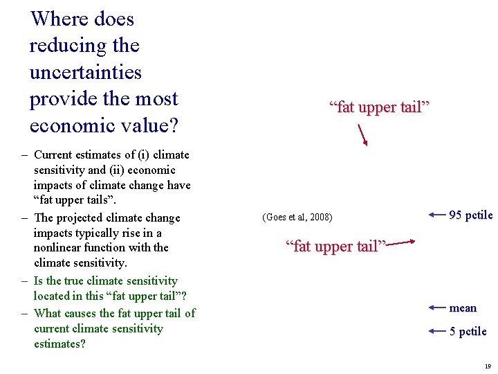
Where does reducing the uncertainties provide the most economic value? – Current estimates of (i) climate sensitivity and (ii) economic impacts of climate change have “fat upper tails”. – The projected climate change impacts typically rise in a nonlinear function with the climate sensitivity. – Is the true climate sensitivity located in this “fat upper tail”? – What causes the fat upper tail of current climate sensitivity estimates? “fat upper tail” (Goes et al, 2008) 95 pctile “fat upper tail” mean 5 pctile 19

Deriving Detection and Prediction Times Detection: – Extension of the Santer et al. (1995) bootstrap method to account for uncertainty in observations and the initial conditions. – Simple Frequentist hypothesis testing. – Use the high-sensitivity case to generate potential future observations. – Detection time: When can one reject Ho of the unforced state with p < 0. 05? Prediction: – Bayesian data assimilation using Markov Chain Monte Carlo and the Metropolis Hastings algorithm. – Likelihood function accounting for autocorrelated errors (Zellner, 1964). – Uncertainty is considered about a single parameter (the NA hydrological sensitivity) with prior uniform range (Zickfeld et al. 2004). – Prediction time: When are the predictions to 95% correct about the threshold crossing? This approach neglects several important uncertainties. Considering these uncertainties would likely strengthen our forthcoming conclusions. 20

This example is actually much easier than the real problem. Would observing the MOC intensity alone enable early prediction? 21

Observation systems designed for early detection may fail at the task of early prediction. - Detection and prediction times are random variables. - Early detection may be possible based on MOC observations alone. - Ocean observation systems designed for early detection of MOC changes may be insufficient for confident and early prediction of an MOC collapse. - Why does learning take so long? Keller and Mc. Inerney (2007) 22

Why does learning take so long? - The signal enabling early prediction of an approaching MOC threshold is associated, in this analysis, with the rate at which the MOC intensity decreases. - A faster MOC weakening implies a higher hydrological sensitivity. - A hydrological sensitivity exceeding a critical level results in an MOC threshold response. - The signal-to-noise ratio is very low before threshold is crossed. - How can we improve the signal-tonoise ratio? Keller and Mc. Inerney (2008) 23

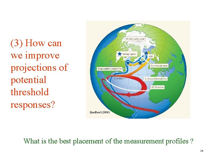
(3) How can we improve projections of potential threshold responses? Quadfasel (2006) What is the best placement of the measurement profiles ? 24

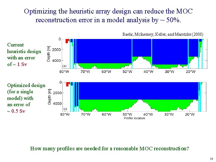
Optimizing the heuristic array design can reduce the MOC reconstruction error in a model analysis by ~ 50%. Baehr, Mc. Inerney, Keller, and Marotzke (2008) Current heuristic design with an error of ~ 1 Sv Optimized design (for a single model) with an error of ~ 0. 5 Sv How many profiles are needed for a reasonable MOC reconstruction? 25

The marginal increase in MOC reconstruction skill drops drastically after just a few profiles. Baehr, Mc. Inerney, Keller, and Marotzke (2008) What about the information contained in biogeochemical tracers? 26

Temporal trends in Apparent Oxygen Utilization may be a useful indicator for a MOC slowdown (combined WOCE A 16 -A 23 sections) – An MOC slowdown is associated with a shoaling of the boundary between Antarctic Bottom Water (AABW) and North Atlantic Deepwater (NADW). – This shoaling results in distinct temporal trends in water mass tracers. – Oxygen observations (and derived water mass tracers) provide (i) a relatively high signal-to-noise ratio, and (ii) a signal in addition to the already used temperature and salinity observations. 27

AOU trends are mechanistically linked to MOC changes and can improve the signal-to-noise ratio. Brennan, Matear, and Keller (2008) How does adding AOU observations affect detection times? 28

Adding AOU to the observation array can reduce the reliable detection time by ~ 20 years. Brennan, Matear, and Keller (2008) What about the other uncertainties? 29

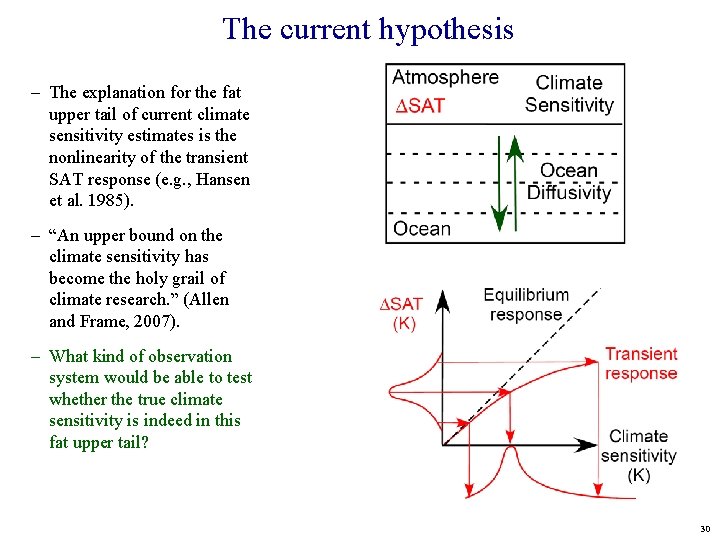
The current hypothesis – The explanation for the fat upper tail of current climate sensitivity estimates is the nonlinearity of the transient SAT response (e. g. , Hansen et al. 1985). – “An upper bound on the climate sensitivity has become the holy grail of climate research. ” (Allen and Frame, 2007). – What kind of observation system would be able to test whether the true climate sensitivity is indeed in this fat upper tail? 30

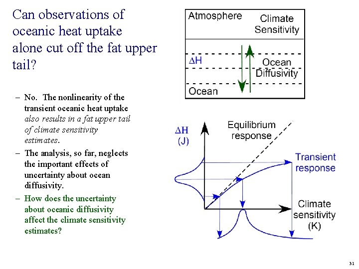
Can observations of oceanic heat uptake alone cut off the fat upper tail? – No. The nonlinearity of the transient oceanic heat uptake also results in a fat upper tail of climate sensitivity estimates. – The analysis, so far, neglects the important effects of uncertainty about ocean diffusivity. – How does the uncertainty about oceanic diffusivity affect the climate sensitivity estimates? 31

Uncertainty about oceanic diffusivity increases the uncertainty in climate sensitivity estimates. – The correlation between climate sensitivity and ocean diffusivity changes sign from the surface air temperature to the and oceanic heat uptake constraint. – Can one use this change in correlation to cut off the fat upper tail of the climate sensitivity estimates? 32

Can the change in correlation between ocean diffusivity and climate sensitivity be used to cut off the fat upper tail? – High climate sensitivity estimates that would be consistent with the surface air temperature record are inconsistent with the oceanic heat uptake. – Likewise, low climate sensitivity estimates that would be consistent with the oceanic heat uptake are inconsistent with the surface air temperature observations. – Combining high precision estimates of the oceanic heat uptake and can, in principle, cut off the fat upper tail of climate sensitivity estimates. – Key caveats: (i) simple model, (ii) we neglect forcing uncertainty. Keller and Urban (2008) 33

The North Atlantic Thermohaline Circulation might collapse at increased radiative forcing Note the physical bifurcation in the THC response to a 2 x CO 2 and a 4 x CO 2 policy. 34 Manabe and Stouffer (1994)